These notes are for the Spring 2021 version of Computer Science 170: Efficient Algorithms and Intractable Problems, based on Algorithms by Christos Papadimitriou, Sanjoy Dasgupta, and Umesh Vazirani.

Midterm 1

Big-O Notation

Runtime is expressed in terms of basic computer steps. For functions $f(n)$ and $g(n)$, we have:

Use the following rules:

1. Multiplicative constants are dropped.
2. For all \(a > b\), \(n^a\) dominates \(n^b\).
3. Any exponential dominates any polynomial.
4. Any polynomial dominates any logarithm.

To demonstrate an asymptotic, compute the limit $\lim_{n \to \infty} \frac{f(n)}{g(n)}$.

Divide and Conquer

Master Theorem

The general format for regression is as follows, where \(a\) is the number of children, \(b\) is the reduction in problem complexity, and \(c\) and \(d\) describe the complexity at each level.

These can be evaluated as:

For complicated recurrence relationships, substitute and expand, examining patterns.

Median

To select the \(k\)th smallest element in an array, repeatedly partition the array by a randomly selected element \(v\). Since there is a 50% chance that the \(v\) is between the 25th and 75th percentile, we expect the array to shrink by 25% after two partition, so the expected running time is

which is \(O(n)\) by the master theorem.

Matrix Multiplication

Subdivide two matrices and multiply as:

This is \(O(n^3)\), which is inefficient. Strassen discovered a way to compute

where

resulting in a new running time of \(T(n) = 7T(\frac{n}{2}) + O(n^2)\) which by the master theorem is \(O(n^{\log_27})\).

Fast Fourier Transform

The FFT expedites the multiplication of two polynomials. For some polynomial \(A(x)\), we pad the polynomial to have \(n = 2^k\) coefficients \(a_0, a_1,..., a_{n-1}\). The FFT outputs the values of \(A(x)\) on the $n$th roots of unity, \(\omega^0, \omega^1,..., \omega^{n-1}\) where \(\omega = e^{2\pi i/n}\).

The algorithm divides the polynomial into even coefficients \(A_e = a_0, a_2, ..., a_{n-2}\) and odd coefficients \(A_o = a_1, a_2, ..., a_{n-1}\). We recursively call \(FFT(A_e, \omega^2)\) and \(FFT(A_o, \omega^2)\). Notice that \(\omega^2\) corresponds to the \(n/2\)th roots of unity, so we can assign the results to \(A_e^{k}\) and \(A_o^{k}\) for \(0 \leq k \leq n/2\).

The results are recombined as \((A^i) = A_e(\omega^{2(i \mod n/2)}) + \omega^{i}A_o(\omega^{2(i \mod n/2)})\) for \(0 \leq i \leq n\).

Now, for two polynomials \(A(x)\) and \(B(x)\), we compute the polynomials on the \(n\) roots of unity using \(FFT\) and compute \(C(x)\) on those points. Surprisingly, we can interpolate by computing \(FFT(C, \omega^{-1})\), yielding a result in \(O(n, \log n)\) operations.

Graphs

Representation

A graph is most commonly represented as an adjacency matrix or adjacency list. For a graph of \(n\) vertices and \(e\) edges, a matrix requires \(O(n^2)\) space but provides constant access. A list requires just \(O(e)\) and \(O(n)\) access.

DFS

Depth first search (DFS) involves repeatedly calling the explore procedure on unvisited starting points until the entire graph has been traversed. It marks each visit with a pre/post-visit number and explores every edge, resulting in a runtime of \(O(v+e)\). In an undirected graph, DFS can be used to identify connected components.

In DFS, for any two intervals \([pre(u), post(u)]\) and \([pre(v), post(v)]\), either one contains the other or they are disjoint. In the case of the former, the node of the containing interval is the ancestor of the other node.

DAG

A cycle is a circular path. A DAG is a directed, acyclic graph. If a DFS reveals a back-edge, then a directed graph contains a cycle. In a DAG, every edge leads to a vertex with a lower \(post\) number. Every DAG must contain at least one source—no incoming edges—and one sink—no outgoing edges.

In a directed graph, a strongly connected component has the property that for any two nodes \(u\) and \(v\), there exists a path from \(u\) to \(v\) and a path from \(v\) to \(u\). Shrinking a directed graph’s SCCs to nodes produces a DAG since any cycle would constitute a SCC. Therefore, every direct graph is a DAG of its SCCs.

BFS

Breadth-first search partitions a graph into layers emanating from a starting vertex \(s\). For each new layer, the nodes are processed via FIFO. The overall running time is identical to DFS \(O(v+e)\). BFS does not restart in other connected components, so nodes unreachable from \(s\) are ignored.

When edges have unit length, an edge of length \(l\) could just be broken down into \(l\) weightless edges. But, this is silly. Dijkstra’s algorithm uses a priority queue to repeatedly explore the most proximate edge. The running time is identical to BFS, but is slowed down by the use of a priority queue. With a heap, the running time is \(O((v+e)\log v)\).

When there are negative edges, we can no longer use Dijsktra’s, since distance is no longer strictly increasing. Instead, we use Bellman-Ford, which “updates” every edge \(v-1\) times. If there is a finite shortest path, then it must be reachable with \(v-1\) nodes. If there a negative cycle, then it doesn’t make sense to ask about a shortest path. We know there is a shortest cycle is distance is reduced on the \(v-1\)th update.

Stacking

Some problems can be simplified by “stacking” multiple copies of a given graph. For example, suppose we want to construct a walk on graph \(G\) that crosses a given edge \((u, v)\) four times before returning to starting node \(s\). We can create five copies of \(G\), with each edge replaced wtih \((u_i, v_{i+1})\), and run Dijkstra’s the compute the shortest distance from \(s_0\) to \(s_4\).

Greedy Algorithms

Greedy algorithms solve a problem by making immediately optimal decisions at each step. In the cases of MSTs, Huffman encoding, and Horn formulas, greedy produces optimal solutions. In the case of set cover, it produces a decent approximation. And in the case of chess, it’s a shit strategy (I can prove this fact with first-hand experience).

To prove a greedy algorithm is optimal, use a proof by contradiction. Assume that a given piece of the optimal solution disagrees with the greedy solution and show that it leads to a contradiction.

MSTs

Greedy algorithms can correctly construct minimum spanning trees, an algorithm called Krustal’s algorithm. Begin at any node and repeatedly add the edge of lowest weight that doesn’t produce a cycle.

Correctness is demonstrated by the cut property. Across any cut of an MST, the lowest weight edge \(e\) is included in a valid MST. This must be the case, since \(e\) is of equal or lower weight the current edge over the cut, \(e'\).

Midterm 2

Greedy

Huffman Encoding

Tasks like audio compression involve efficiently representing a string. Suppose it need to encode an alphabet of characters \(A\), \(B\), \(C\), and \(D\). We could create a unique 2-bit representation of each. But if one of the character is predominant in the string, such an encoding would be inefficient. We want to define binary codewords of different lengths, and we can do so with a full binary string.

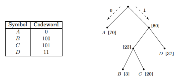
For a given tree of \(n\) symbols, each with frequency \(f_i\) and depth \(d_i\), we can compute the cost of the tree as \(\sum^n_{i=1} f_i * d_i\). Equivalently, the cost is the sum of the frequencies of all leaves and internal nodes, excluding the root.

We can construct this tree greedily using Huffman encoding. Iterate through a priority queue of frequencies in ascending order. Remove the two smallest frequencies \(f_i, f_j\) and add \(f_k = f_j + f_i\) to the priority queue. Then, create a node \(k\) with children \(i, j\).

Horn Formulas

A Boolean variable is either true or false and a literal is either a variable or its negation. Horn formulas store knowledge in two forms of clauses. Implication clauses state that a combination of positive literals imply a single positive literal, e.g. \((z \land w) \implies u\). To dictate that a variable is always true, remove the predicate, e.g. \(\implies x\). Negation clauses take the form of “at least one must be false”, e.g. \(\neg a \lor \neg b \lor \neg c\).

We can use a greedy algorithm to find a satisfying assignment of true and false values. Begin by setting everything false. Then, while there exists an unsatisfied implication, set the consequence to true. If all negative clauses are met, return the assignment. Otherwise, the clauses are inconsistent.

Set Cover

Suppose we are given a group of sets \(S_0, S_1, S_2, ..., S_n\) and a target set of elements \(B\). How can we select the minimal number of sets to cover the target set? A greedy approach would repeatedly pick the smallest set \(S_i\), but it doesn’t guarantee optimality. To see this, consider the following set.

Fortunately, greedy can still provide a good approximation. Suppose \(B\) contains \(n\) elements and the optimal cover includes \(k\) sets. In picking each set, the number of remaining uncovered elements \(n_t\) decreases by at least \(\frac{n_r}{k}\). This implies that \(n_t \leq n(1-1/k)^t \leq ne^{-t/k}\).

Dynamic Programming

Dynamic programming and linear programming are “sledgehammers,” techniques that provide broad applicability at the expense of efficiency.

Shortest Paths

Shortest paths are easy to find in DAGs because the nodes can be linearized, arranging them on a line so that the edges go left to right. The algorithm happens to be an example of dynamic programming. For a given node, we break the problem down by finding the shortest path to every incoming node.

Longest Increasing Subsequence

Given a sequence of numbers \(a_1, a_2, ..., a_n\), an increasing subsequence is any strictly increasing ordered subset. Notice that comparisons produce a similar structure to a dag.

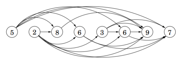
We use a similar approach. Begin the subsequence at each index and consider the longest subsequence from each subsequent node of greater value.

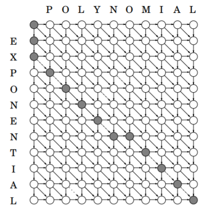
Edit Distance

Suppose we have two strings. The edit distance between the strings is the minimum number of insertions, deletions, and substitutions to get from the first string to the second.

We can break this down into subproblems by considering the edit distance between the first \(i\) characters of the first string and the first \(j\) characters of the second string. We can either delete the \(i\)th character of string one, add the \(j\)th character of string two, or substitute the \(i\)th character. It corresponds to the following recurrence relationship: \(E(i, j) = \min[1 + E(i-1, j), 1+E(i, j-1), \text{diff}(i, j) + E(i-1, j-1)]\) Underlying the solution is a DAG with edges from different combinations of \((i, j)\).

Knapsack Problem

We have a set of \(n\) items form which to choose, each of which has weight \(w_i\) and value \(v_i\). We want to maximize the value subject to the capacity \(w\). If we are allowed to repeatedly pick items, then we can repeatedly pick the item which maximizes the value, notated as \(K(w) = \max_{i:w_i\leq w} \{K(w-w_i) + v_i \}\) But, if we are not allowed to repeat items, then we must introduce a second parameter \(0 \leq j \leq n\), where \(K(w, j)\) is the maximum value achievable using a knapsack of capacity \(w\) and items \(1, ..., j\). We have the new recursive relationship: \(K(w, j) = \max \{K(w-w_j, j-1) + v_j, K(w, j-1) \}\) To avoid repetition of subproblems, we use memorization, storing the solutions to subproblems that we’ve already seen. The running time is \(O(nW)\).

Chain Matrix Multiplication

Suppose we have a chain of matrices \(A_1 \times A_2 \times ... \times A_n\) with dimensions \(m_0 \times m_1, m_1 \times m_2, ..., m_{n-1} \times m_n\). We can represent the order of multiplication with a binary tree, such as below.

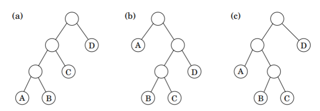
Given a list of dimensions, we can set up a recurrence relationship for matrices \(i\) through \(j\) by choosing the cheapest pair \(k, k+1\) to multiply first: \(C(i, j) = \min_{i\leq k \leq j} \{C(i, k) + C(k+1, j) + m_{i-1} \cdot m_k \cdot{} m_j\}\) The algorithm runs in \(O(n^3)\), with \(O(n^2)\) subproblems that take \(O(n)\) to compute each.

Shortest Paths

Suppose we want to find the shortest path from node \(s\) to every other path with at most \(k\) edges. We can modify the Dijkstra’s update function as follows: \(\text{dist}(v, i) = \min_{(v, u)\in E} \{\text{dist}(u, i-1) + l(u, v) \}\) But if we want to find the shortest path between every pair of vertices, we can use a faster algorithm. We instead let \(\text{dist}(i, j, k)\) denote the length of the shortest path from \(i\) to \(j\) where only the nodes \({1, 2, ..., k}\) can be used as intermediates. Updating is easy, since we just to need examine whether adding the \(k\)‘th node presents a shorter path for some \(i\) and \(j\) with an edge to \(k\). In other words, we update: \(\text{dist}(i, j, k) = \min \{\text{dist}(i, k, k-1) + \text{dist}(k, j, k-1), \text{dist}(i, j, k-1)\}\) with a runtime of \(O(\|V\|^3)\), which is better than the \(O(\|V\|^2 \|E\|)\) we’d get from running Dijkstra’s from each node.

Traveling Salesman

Suppose we want to find a tour between \(n\) nodes which visits every node exactly once and has minimum total length. A brute force solution checking every possible tour would take \(O(n!)\) time. Instead, we can evaluate every subset of size \(s\) that contains a starting node \(j\). We iterate through subsets \(S\) in ascending order of size \(s\) and all nodes, updating: \(C(S, j) = \min \{C(S - \{j\}, i) + d_{ij} : i\in S, i\neq j\}\) The \(2^n \cdot n\) subproblems each are linear time, so the running time is \(O(n^2 2^n)\).

Linear Programming

Overview

An optimization problem consists of \(n\) variables \(x_1, x_2, ..., x_n \in \mathbb{R}\), an objective function \(f(x_1, x_2, ..., x_n) \in \mathbb{R}\), and \(m\) constraints \(C_1, c_2, ..., c_m\) with \(c_i(x_1, x_2, ..., x_n) \in \mathbb{R}\). The goal is to maximize \(F\) subject to every \(c_i\).

A linear programming problem involves a linear \(f(x_1, x_2, ..., x_n) = a_1x_1 + ... + a_nx_n\) with \(a_1, ..., a_n \in \mathbb{R}\) and a set of linear constraints (e.g. \(x_1 + x_2 = 1\) or \(x_3 - 4x_4 \geq 5\)). Strict inequalities are not allowed because the set of possible solutions would not be topologically closed. A generic setup can be written as: \(\max e^T x\\ Ax \leq b\\ x \geq 0\)

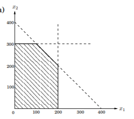
Visually, a set of constraints forms a region of feasible solutions. This region could be empty or unbounded. If it isn’t, then the region is convex. This is means that if \(\vec{x}\) and \(\vec{y}\) are feasible then so is any \(\vec{z} = \lambda \vec{x} + (1-\lambda) \vec{y}, \forall \lambda \in [0, 1]\). The conclusion is that any point on the interior can improve and any point on the edge can move along to a vertex.

Simplex

Simplex is a greedy strategy that begins with any vertex and moves to adjacent vertices. Each vertex is defined by \(n\) constraints at equality, and an adjacent vertex involves relaxing a constraint and tightening another constraint.

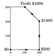
The correctness follows from convexity. Suppose that at some vertex \(v\), each of its neighbors has the same or worse value. Then, the feasible region is below the profit line going through \(v\).

The runtime is exponential. There are \({m \choose n}\) vertices, so while simplex halts in finite time, the above bound is exponential.

Network Flow

Suppose we wish to maximize the “flow” through a network subject to constraints on flow through each edge.

We reduce the problem to linear programming for the variables \({f(e)}_{e \in E}\) with constraints \(0 \leq f(e) \leq c(e)\) and \(\sum f(u, v) = \sum f(v, w)\) for all \(e\) and \(v\) with an objective function of \(\sum f(s, u)\) where \(s\) is the source. Solving the generic LP problem gives us a polynomial time solution.

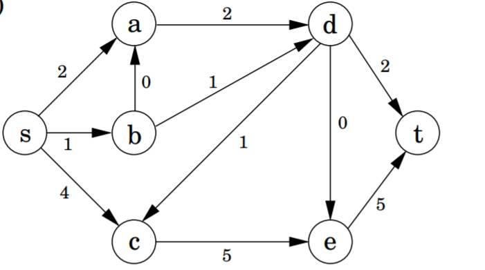
A direct algorithm can solve the problem by modifying greedy. Begin with zero flow and repeatedly pick any path, increasing the flow by the maximum amount possible and canceling out existing flow when they travel in opposing directions. Each iteration is \(O(E)\). By the Ford-Fulkerson algorithm with random paths, there are at most \(f_{\max}\) iterations, so the runtime is \(O(E \cdot f_{\max})\). By the Edmunds-Korp algorithm based on BFS, there are at most \(O(V\cdot E)\) iterations and the overall runtime is \(O(V \cdot E^2)\).

The direct algorithm is correct by the Max-Flow Min-Cut Theorem. \(\max f = \min_{\text{cut}(L, R)} \text{capacity}(L, R)\) To see this, suppose there is some max flow \(F^*\). Notice that since it is optimal, there is no path \((s, t)\) in \(F^*\). Let \(L\) be every vertex reachable from \(s\) and \(R\) constitute the rest. The capacity of the cut must be \(f*\), since otherwise there would be another path from \(s\) to \(R\), which by construction is impossible.

Duality

In a primal LP problem, we have \(I\) inequalities and \(E\) equalities over \(n\) variables with \(N\) constrained to be non-negative. The dual has \(m = I + E\) variables with only \(I\) non-negative constraints.

The primal LP takes the generic form: \(\max c_1x_1 + ... + c_nx_n\\ a_{i1}x_1 + ... + a_{in}x_n \leq b_i \text{ for } i\in I\\ a_{i1}x_1 + ... + a_{in}x_n = b_i \text{ for } i\in E\\ x_j \geq 0 \text{ for } j \in N\) While the dual LP takes the form: \(\min b_1y_1 + ... + b_ny_m\\ b_{j1}y_1 + ... + b_{jm}y_m \geq c_j \text{ for } j\in N\\ b_{j1}y_1 + ... + b_{jm}y_m = c_j \text{ for } j\not\in N\\ y_i \geq 0 \text{ for } i \in I\) Weak duality states that the solution to the primal LP problem is always less than or equal to the solution to the dual LP problem. Strong duality states that the solutions are equal.

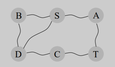
To get the intuition for why this works, consider the shortest path problems between two nodes \(S\) and \(T\) in a graph. Suppose we built a physical model where physical nodes are connected via loose strings. Clearly, we can find the shortest distance by pulling \(S\) and \(T\) away from one another, turning a minimization problem into a maximization problem.

Final

Linear Programming

Zero-sum Games

Suppose two players, Row and Column, are playing rock, paper, scissor. The matrix of outcomes looks as follows:

Clearly, if either player knows their opponent’s move ahead of time, then they can always win. Suppose instead that Row has a mixed strategy, picking \(r, p, s\) with probabilities \(x_1, x_2, x_3\), respectively. We denote Row’s mixed strategy \(x = (x_1, x_2, x_3)\) and Column’s mixed strategy \(y = (y_1, y_2, y_3)\). The expected payoff for a given round is: \(\mathbb{E}[P] = \sum_{i, j} G_{ij}x_iy_j\) If Row adopts a complete random strategy with \(x = (1/3, 1/3, 1/3)\), then it is easy to show that for any choice Column makes, the expected value is 0. In fact, no matter which player goes first, the other can pick \((1/3, 1/3, 1/3)\) and set the EV to 0.

Now consider an asymmetric game, where Row chooses between \(e\) and \(s\) while Column chooses between \(m\) and \(t\).

Notice that for any fixed Row strategy—say, \(x = (1/2, 1/2)\)—there is a pure strategy from Column that is optimal—in this case, \(y = (0, 1)\). Therefore, Row should pick a strategy that maximizes the optimal response from Column: \(\max_{x_1, x_2} \min(3x_1 - 2x_2, -x_1 + x_2)\) But, this is an LP problem: \(\max z\\ -3x_1 + 2x_2 \leq z\\ x_1 - x_2 \leq z\\ x_1 + x_2 = 1\\ x_1, x_2 \geq 0\) Now, notice that Column faces a symmetric problem: \(\min_{y_1 , y_2} \max(3y_1 - y_2, 2y_1 + y_2)\) which we can rewrite as \(\min w\\ 3y_1 - y_2 \leq w\\ -2y_1 + y_2 \leq w\\ y_1 + y_2 = 1\\ y_1, y_2 \geq 1\) These two LPS are dual to one another, so they produce the same optimum \(V\), which is the value of the game.

A more general game theory result is the min-max theorem, which states that \(\max_x \min_y \sum_{i,j} G_{ij}x_iy_j = \min_y \max_x \sum_{i, j} \sum G_{i, j} x_i y_j\)

Multiplicative Weights

Each day, we allocate \(x_i^{(t)}\) of our capital to stock \(i\) on day \(t\). Let \(l_i^{(t)}\) denote the loss we incur on day \(t\) if we invested everything on stock \(i\). At the end of day \(T\) we have lost a total of \(\sum^T_{t=1} \sum^{n}_{i=1} x_i^{(t)}l_i^{(t)}\) On each day, we must pick an array \(x^{(t)} = [x_1^{(t)}, ..., x_n^{(t)}]\) with non-negative \(x_i^{(t)}\) that sum to 1.

Define the regret \(R_T\) on day \(T\) as the difference between the overall loss and the optimal fixed allocation strategy:

\(R_T = \sum^T_{t=1} \sum^n_{i=1} x_i^{(t)} \cdot l_i^{(t)} - \min_{x \text{ probability distribution}} \sum^T_{t=1} \sum^n_{i=1} x_i l_i^{(t)}\) \(= \sum^T_{t=1} \sum^n_{i=1} x_i^{(t)} \cdot l_i^{(t)} - \min_{i = 1, ..., n} \sum^T_{t=1} l_i^{(t)}\)

The multiplicative weight algorithms bounds \(R_T \leq 2\sqrt{T \ln n}\), noticing that \(\frac{R_T}{T} = O(\sqrt{\frac{\ln n}{T}})\). Begin by setting a parameter \(0 \leq \epsilon \leq 1/2\) with weights \(w^{(t)} = [w_1^{(t)},...,w_n^{(t)}]\) where: \(w_t^{(0)} = 1\\ w_i^{(t+1)} = w_i^{(t)} \cdot (1-\epsilon)^{l_t^{(t)}}\) which causes strategies with high losses to lose weight. At each step, the algorithm allocates proportionately to the weights: \(x_i^{(ta)} = \frac{w_i^{(t)}}{\sum_j w_j^{(t)}}\) Let \(L^*\) denote the offline optimum. First, notice that \(W_{T+1} \geq (1-\epsilon)^{L^*}\). Second, we can prove that \(W_{t+1} \leq W_t \cdot (1-\epsilon L_t)\). Taken together, we have: \(\sum^T_{i=1} L_t - L^* \leq \epsilon L^* + \frac{\ln n}{\epsilon} \leq \epsilon T + \frac{\ln } { \epsilon}\) were we can set the terms equal with \(\epsilon = \sqrt{\frac{\ln n}{T}}\), yielding our regret bound.

Reductions

When a subroutine of task \(Q\) is used to solve \(P\), then \(P\) reduces to \(Q\). Visually,

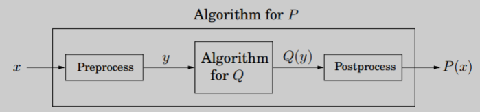
A fast algorithm for \(Q\) provides a fast algorithm for \(P\). But, if \(P\) is hard, then \(Q\) must also be hard.

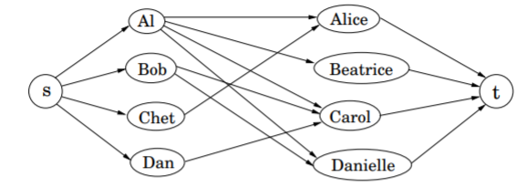
Bipartite Matching

Suppose in a graph with an equal number of boys and girls, an edge a heterosexual crush. A perfect matching is a bipartite matching of the graph and can be reduced the following network flow. The solution is integer since all the edge weights are also integer.

Circuit Value Problem

Suppose we have a Boolean circuit with input gates (value true or false), AND/OR gates with indegree 2, and NOT gates with indegree 1. One gate is called the output. The problem can be reduced to a linear program by creating constructs for each gate.

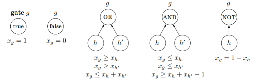
Surprisingly, since any algorithm is ultimately a Boolean circuit, all problems that can be solved in polynomial time also reduce to linear programming.

Matrices

Matrix multiplication (MM) and matrix inversion (MI) reduce to one another.

First, notice that MM reduces to MI because to multiply matrices \(A\) and \(B\), we construct a larger matrix and compute: \(X = \begin{bmatrix}I & A & 0\\ 0 & I & B\\0 & 0 & I \end{bmatrix}\\ X^{-1} = \begin{bmatrix}I & A & AB\\ 0 & I & B\\0 & 0 & I \end{bmatrix}\) yielding our desired result.

Second, we reduce MI to MM through Gaussian elimination: \(\begin{bmatrix}A & B\\ C & D\end{bmatrix} = \begin{bmatrix}I & 0 \\ CA^{-1} & I\end{bmatrix} \cdot \begin{bmatrix}A & B \\ 0 & D - C \cdot A^{-1} \cdot B\end{bmatrix}\) Let \(X = D - C \cdot A^-1 \cdot B\), \(Y = CA^-1\), and \(Z = -A^{-1} \cdot B \cdot S^{-1}\). We easily compute the inverse as: \(\begin{bmatrix}A & B\\ C & D\end{bmatrix}^{-1} = \begin{bmatrix}A & B\\ 0 & S\end{bmatrix}^{-1} \cdot \begin{bmatrix}I & 0\\ Y & I\end{bmatrix}^{-1} = \begin{bmatrix}A^{-1} - Z \cdot Y & Z\\ -S^{-1} \cdot Y & S^{-1}\end{bmatrix}\) Computing \(A^{-1}\) and \(S^{-1}\) are \(F(n/2)\), while computing \(Y\), \(YB\), \(S\), \(Z\), \(Z \cdot Y\) and \(S^-1 \cdot Y\) each take \(O(n^2)\). \(F(n) = 2F(n/2) + O(n^2) = O(n^2)\) by the recurrence master theorem.

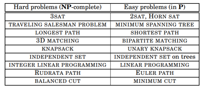
NP-Completeness

Search Problems

A search problem involves an instance \(I\) with a target solution \(S\) that can be quickly verified by a checking algorithm \(C\). The running time is polynomial in \(I\). The class of all search problems is called NP (non-deterministic polynomial time). Meanwhile, the class of all search problems solvable in polynomial time is P. We can leverage reductions to show that certain problems are NP-complete.

SAT

SAT (or satisfiability) involves a boolean formula in conjunctive normal form where several or clauses are and-ed together. We can quickly check if a particular assignment is valid, but it’s hard to check all assignments. If all clauses contain at most one positive literal, then we have a Horn formula which we can check with a greed algorithm. In 2-SAT, where each has only two literals, we can solve it in linear time with SCCs.

We can reduce 3-SAT to independent set as follows. Create a graph with a triangle for each clause and edges between opposite literals. Set the goal \(g\) to the number of clauses. Any solution \(S\) will never contain a contradiction, so it must solve 3-SAT. Conversely, for any solution to 3-SAT, simply add any true literal in each clause to the set \(S\).

We can reduce SAT to 3-SAT as follows. Whenever a clause has more than three literals such as \((a_1 \lor a_2 \lor ... \lor a_k)\), replace it with \((a_1 \lor a_2 \lor y_1) (\bar{y_1} \lor a_3 \lor y_2) (\bar{y_2} \lor a_4 \lor y_3) ... (\bar{y}_{k-3} \lor a_{k-1} \lor a_k)\) If this version is satisfied, then it is easy to see that the original must be satisfied. Conversely, if some \(a_i\) is true, then we can set \(y_1, ..., y_{i-2}\) to true and the rest to false.

Any problem in NP reduces to SAT because we can generalize SAT to Circuit SAT, which has AND/OR/NOT gates, known inputs, and unknown inputs. SAT can trivially be represented as a Circuit SAT with no known input gates. In the other way around, we can represent OR, AND, and NOT by breaking them down into one or more clauses.

TSP

The Traveling Salesman Problem looks for a tour among \(n\) vertices with total cost constrained by budget \(b\). We introduce the constraint so we can reduce the optimization problem (which can’t be checked in polynomial time) to a search problem. We can use a binary search on the budget to find the optimal cost. There are only exponential time algorithms for TSP.

Rudrata

Two twin problems are the Rudrata cycle–which visits each vertex exactly once—and Euler cycle—which traverse each edge exactly once. Rudrata cycle is not solvable in polynomial time because it focuses on vertices.

Rudrata path is equally hard. Suppose we have an instance of Rudrata path from \(s\) to \(t\). Create new edges \((s, x), (x, t)\). This trivially reduces to Rudrata path.

Rudrata can be reduced to TSP as follows. Construct an instance of TSP with unit length edges and \(1+\alpha\) length edges where they aren’t suppose to exist. For \(\alpha = 1\), we have the triangle inequality.

ILP

There is no efficient algorithm for integer linear programming, where we are given a set of linear inequalities \(AX \leq b\).

ZOE can be reduced to subset sum by turning each column’s elements into digits. ZOE can be reduced to ILP by constraining each variable to be between 0 and 1.

3D Matching

Given a tripartite graph with \(n\) nodes on each side, find \(n\) disjoint edge triples or decide that none exists. We can reduce 3-SAT to 3D matching by using this gadget.

We can then link up clauses by pairing the pets and adding extra boys and girls to fill in the gaps.

We can easily reduce 3D matching to ZOE via the following matrix.

Set, Cover, Clique

In Independent Set, given a graph and integer \(g\), find \(g\) independent vertices (which share no edge). It can be solved efficiently on trees, but not for general graphs. In Vertex Cover, the goal is to find \(b\) vertices which \(b\) vertices that touch every edge. Vertex Cover and 3D matching are both special cases of Set Cover.

We reduce Independent Set to Vertex Cover by computing the vertex cover on \(\|V\|_g\) nodes. Notice that the complement must be an independent set.

We reduce Independent Set to Clique by checking if a set of nodes \(S\) in \(G\) is a clique in \(\bar{G}\).

Longest Path

Find a simple path from \(s\) to \(t\) with weight at least \(g\).

Knapsack

Knapsack is exponential in its input size since it looks at every subset. The unary knapsack variant has an efficient solution. A seemingly simple variant called Subset Sum—where each item’s value is its weight and we wish to reach a capacity—is also hard.

Dealing with NP-Hard

Approximation

For any minimization problem, the approximation ratio of the algorithm is defined to be \(\alpha_A = \max_I \frac{A(i)}{\text{OPT}(I)}\) which is to say, a factor by the which the output exceeds the optimal solution.

We can approximate vertex cover with a matching, a subset of edges with no vertices in common. Repeatedly add disjoint edges until no longer possible. It is guaranteed to have at most 100% error, so \(\alpha_A = 2\).

Not all NP-hard problems have approximation ratio 2 . For example, if TSP has an approximation ratio of 2, then we could solve Hamiltonian Cycle by adding a length 2n edge on all non-existing edges. An algorithm with approx. ratio 2 could tell the difference.

Heuristics

To find the maximum of a function \(f\), we should follow the up direction, which is called gradient ascent. The idea is to pick a random starting point \(z\) and try to find a better point \(z'\) near \(z\) over \(M\) iterations. It gets close to gradient descent when we choose worse option according to an exponential decaying temperature schedule.

Randomized Algorithms

Consider a quicksort of array \(A\) with random pivots. The worst case will have an empty left or right and fail to divide. The best case is divide and conquer. Using an indicator variable, we can show that the expected value of each comparison \(X_{ij}\) between entry \(i\) and \(j\) has an expected value \(\mathbb{E}(X_{ij}) = \frac{2}{j-i+1}\). Summing across all \(i, j\), we have \(2n\log n\).

Freivalds’ Algorithm gives a quick way of testing if \(C = A \times B\) by picking a uniformly random \(x \in {0, 1}^n\). If \(C = A \times B\), then \mathbb{P}(ABx = Cx) = 1\(. Otherwise,\)\mathbb{ABx = Cx} \leq 1/2\(. To show the latter, consider\)D := AB - C\(and notice that at most half of all\)Dx\(could be 0. If we pick\)N\(random and independent vectors, then the probability of failure is\)\frac{1}{2^N}$$.

Karger’s Global Minimum Cut algorithm uses contractions. The algorithm uniformly contracts an edge (replacing it with a supervertex) \(V-2\) times. The probability that Contraction returns the global minimum is at least \(\frac{1}{n \choose 2}\). This happens if no edge crossing the cut is contracted. The probability expression is a telescoping product that equals \(\frac{1}{n \choose 2}\). Using the fact that \(1+x \leq e^x\), we can compute that repeating the algorithm \(N\) times has a \(O(mN) = O(mn^2\log(1/p))\) runtime.

Streaming

Suppose we want a data structure that can approximately count with error bound \(\mathbb{P}(\text{abs}(\tilde{n} - n) > \epsilon n) < \delta\) A trivial algorithm would use log(n) memory. While we could instead only increment \(X\) with probability \(1/2\), the memory saving is small and the approximation is bad for small \(X\). Morris devised this algorithm:

1. Initialize \(X = 0\)
2. For each update, increment \(X\) with probability \(\frac{1}{2^X}\).
3. Output \(\tilde{n} = 2^X - 1\).

Using induction, we can show \(\mathbb{E} 2^{X_n} = n+1\). By using \(s\) copies of Morris and averaging them, we can reach \(\mathbb{P} (\text{abs}(\tilde{n} - n) > \epsilon n) < \frac{1}{2s\epsilon^2}\).

Lower Bounds

Any comparison based sorting algorithm takes at least \(\omega(n \log n)\) time. Since there are \(n!\) possibilities for the true sorted order, there are at least \(\log (n!)\) decisions it needs to make.

We haven’t found a superlinear lower bound for any explicit problem. Cell probe lower bounds are the gold standard since they only count read and write. Everything else is free!

Hashing

We hash using $h_a (x_1, x_2…, x_k) = \sum^k_{i=1} a_i x_i \mod n$ and are guaranteed a chance of collision of 1/n. We picked a random hash function by drawing the \(a_i\), so they are universal.

Probability

Markov’s inequality for a nonnegative random variable \(X\): \(P(X \geq a) \leq \frac{E(x)}{a}\) Chebyshev’s inequality guarantees that \(P(|X-\mu| \geq c) = P((X-\mu)^2 \geq c^2) \geq \frac{\sigma^2}{c^2}\)