These notes are for Summer 2021’s Economics 119: Psychology and Economics.

Choice

There are four types of choice problems:

1. Choice under certainty: pick your favorite.
2. Choice under uncertainty: pick your favorite gamble.
3. Choice over time: pick your favorite consumption stream.
4. Choice under strategic interaction: pick your favorite action in the presence of others.

The standard model involves a rational decision maker (DM) that…

• maximizes a utility function.
• discounts the future.
• evaluates risk using expected utility theory.
• thinks recursively in strategic situations.
• is selfish.
• applies Bayes’s rule to form beliefs.

Rationality involves ‘Selecting the most preferred from the available options’. Mathematically, we can write \(\max{U} \text{ subject to } B\) or, under uncertainty, \(\max{EU} \text{ subject to } B \\ EU(L) = \sum^N_{n=1} u_n p_n\) The key question is: what can explain the choices people make? And, are these choices consistent?

Economics is done in three ways:

1. Theory, which uses mathematical models to draw conclusions from a set of assumptions.
2. Experiments, which test hypotheses in both the lab and the field.
3. Empirical analysis, involving the statistical modeling of real world data, often drawing on interesting natural experiments.

Models tell stories. They can never be fully realistic, but they can provide useful insights. For example, we usually assume that someone will choose as if they were rational. One key tradeoff is between the level of detail and the breadth of applicability. Don’t chase realism - the world is not the model, and the model is not the world.

The rest of the course is divided into the topics of choice, time, risk, games, fairness, and beliefs.

Choice

Standard Model

The standard model involves objectives and constraints. In our model, a consumer chooses among bundles of goods (which could be, for example, across different time periods). Let \(x_i\) denote the amount of good \(i\) so that a bundle of $n$ types of goods could be \(x = (x_1, x_2, ..., x_{n-1}, x_n)\) People have preferences over bundles that involve an ordering of every conceivable bundle. Some notation:

• \(x \succ y\) - bundle \(x\) is strictly preferred to bundle \(y\)
• \(x \sim y\) - the consumer is indifferent between bundle \(x\) and \(y\)
• \(x \succsim\) - bundle \(x\) is weakly preferred to bundle \(y\)

We make two assumptions about preferences:

1. Completeness: either \(x \succsim y\) or \(y \succsim x\) or both. A consumer can’t “not know.”
2. Transitivity: for all triples \(x, y, z\), we have:
   • if \(x \succ y\) and \(y \succ z\), then \(x \succ z\)
   • if \(x \sim y\) and \(y \sim z\), then \(x \sim z\)
   • if \(x \succ y\) and \(y \sim z\), then \(x \succsim z\)
   • if \(x \sim y\) and \(y \succ z\), then \(x \succsim z\)

Utility Functions

Utility is a tool to help compare bundles and can be notated \(u(x_1, x_2) = f(x_1, x_2)\) for the two-good case. A set of preferences that satisfies completeness and transitivity can be represented such that \(x \succsim y\) if and only if \(u(x) \geq u(y)\). Utility functions are ordinal, not cardinal. An order-preserving transformation of a utility function represents the same preference.

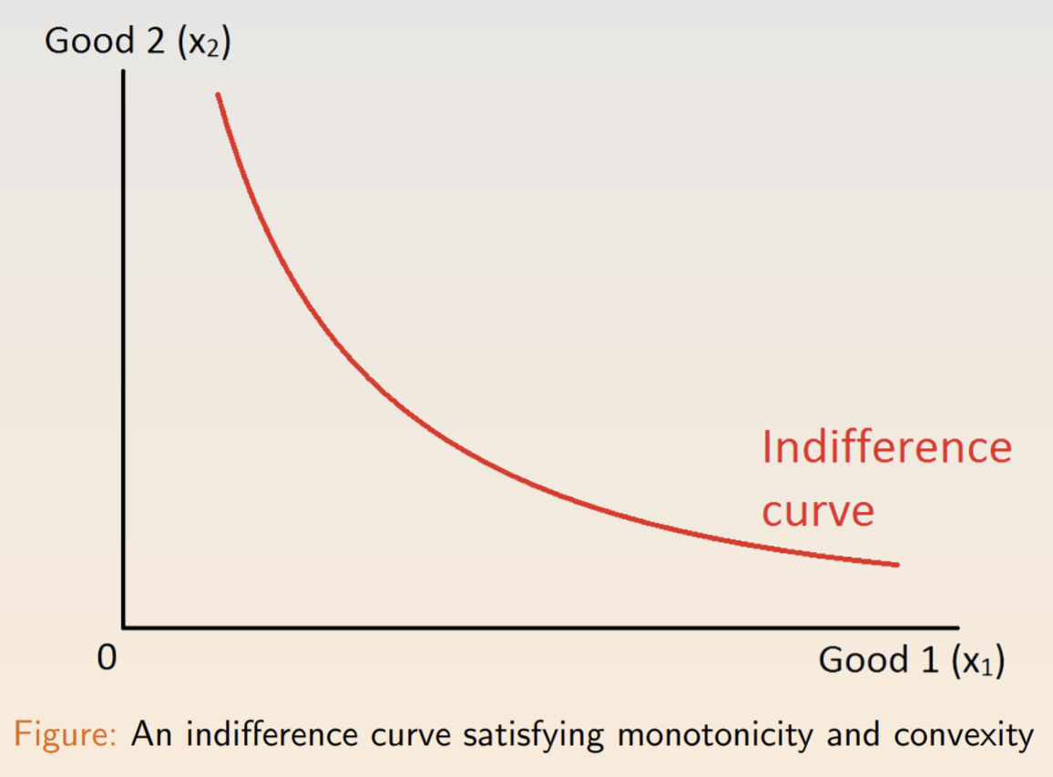
An indifference curve comprises all the bundles with the same utility. In an indifference map, each indifference curve is a level set of the utility function. Preferences are usually assumed to be monotonic (more is better) and convex (bundles on a straight line between two bundles are better). Such a curve is below.

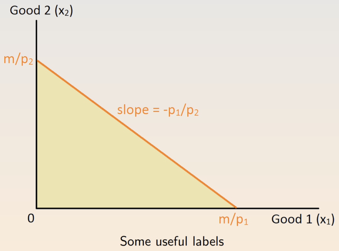
The marginal rate of substitution (MRS) is the rate at which a consumer is willing to trade one good for another. As the size of the exchange gets smaller, the ratio approaches the slope of the indifference curve. We can compute the MRS from marginal utility (MU), so that \(MRS = -\frac{\Delta x_2}{\Delta x_1} = \frac{\delta U / \delta x_1}{\delta U / \delta x_2} \frac{MU_1}{MU_2}\) One common constraint is budgets. For each unit of a good \(x_i\), the customer must pay a price \(p_i\) from an income \(m\). The budget constraint is \(p_1x_1 + p_2x_2 \leq m\).

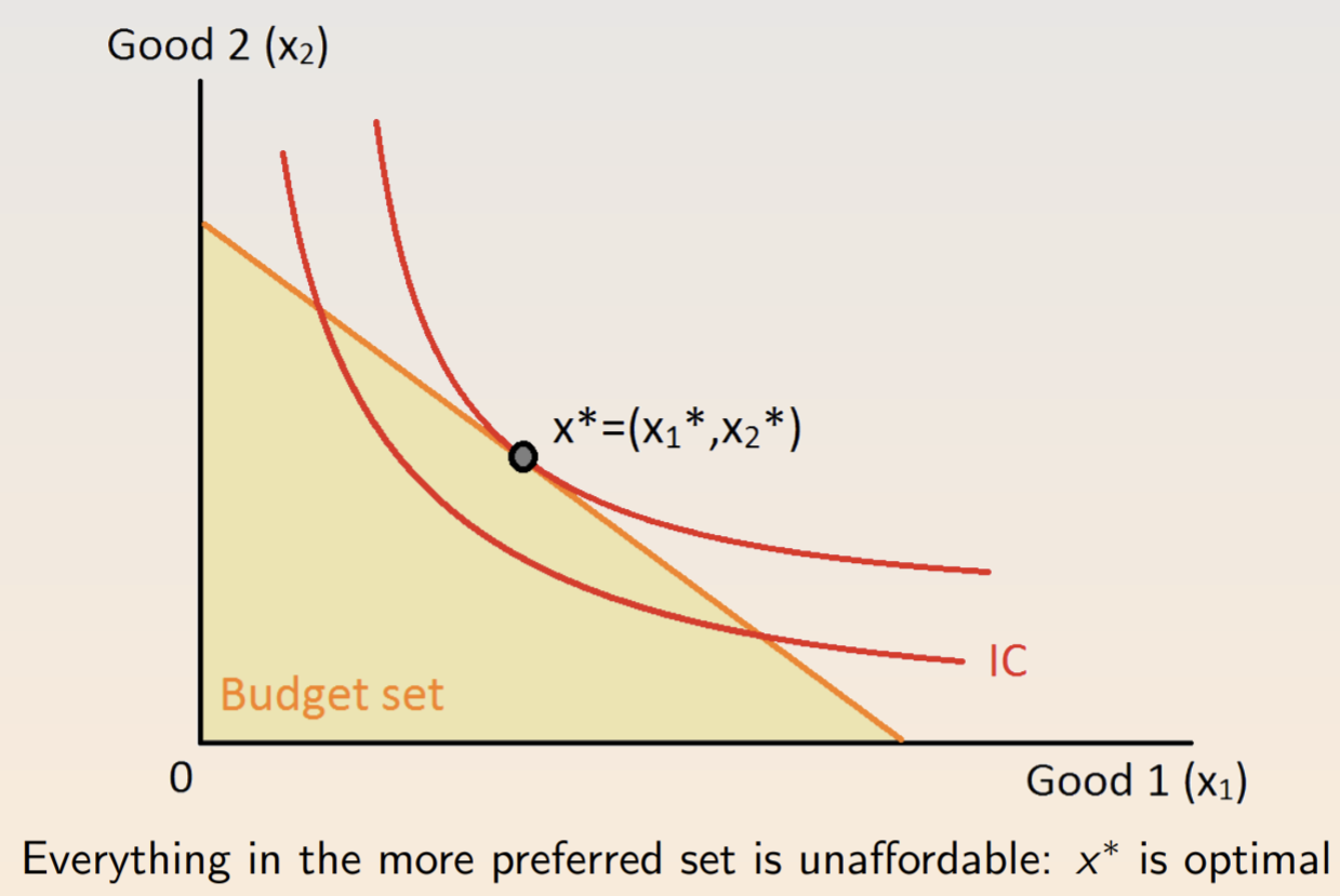
The optimal choice for well-behaved preferences is found at the tangent, where \(MRS = \frac{p_1}{p_2}\). At tangency, there’s no swap that the consumer is willing to make.

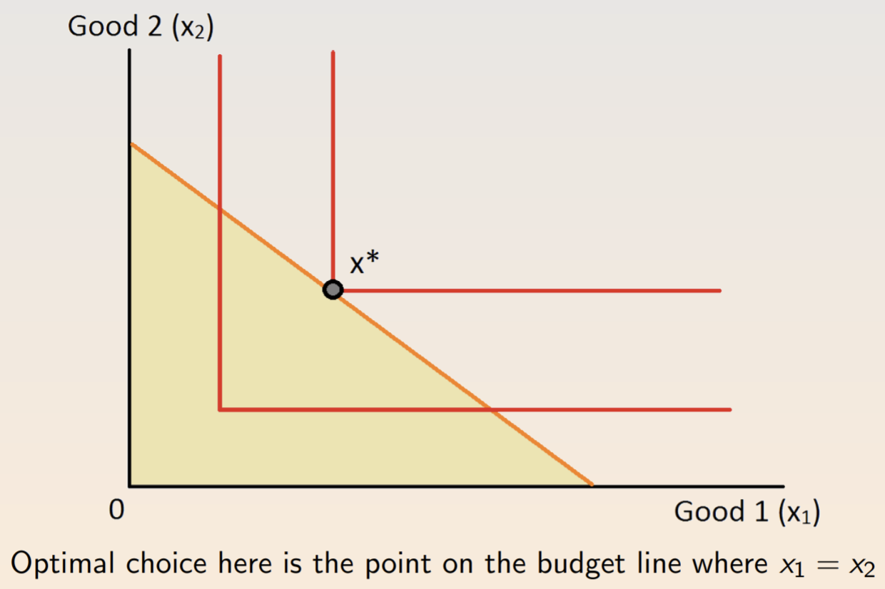
This optimality condition applies in the case of perfect complements….

…and for perfect substitutes.

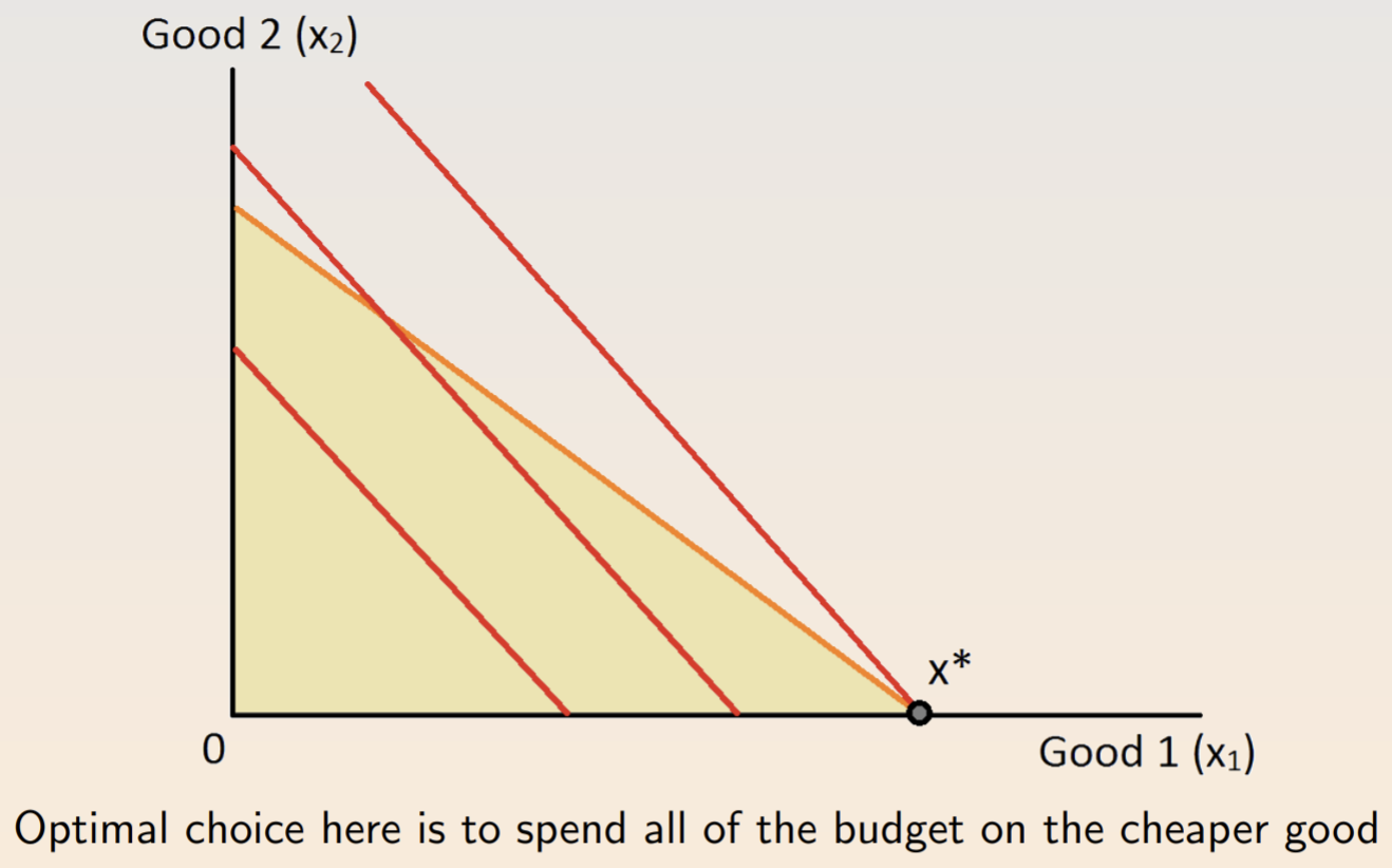
A mathematical analog of the graphical argument is utility maximization: \(\max u(x_1, x_2) \text{ subject to } p_1x_1 + p_2x_2 \leq m\) The constrained optimization problem is the foundation of microeconomics. Again, under monotonic preferences, the constraint will bind the equality at the optimum. There are four ways to solve it:

1. Brute force: solve for one of the variables and substitute it back into the utility function.
2. Tangency: for well-behaved preferences and triangle budgets, the solution is the tangency point, where \(MRS = \frac{p_1}{p_2}\).
3. Lagrangian: compute partial derivatives of the Lagrangian.
4. Art: it’s often easier to sketch the solution, especially if the preferences aren’t well-behaved and there’s a corner solution.

Preferences are assumptions. When you test a model, you also test the underlying preferences. If you have data, you should figure out a target observation and a level of structure.

Rationality

Some properties of rational preferences:

1. The independence of irrelevant alternatives (IIA): If \(x\) is chosen from a set of alternatives \(A\) and \(B\) is a subset of \(A\) that also contains \(x\), then \(x\) must be chosen from \(B\).

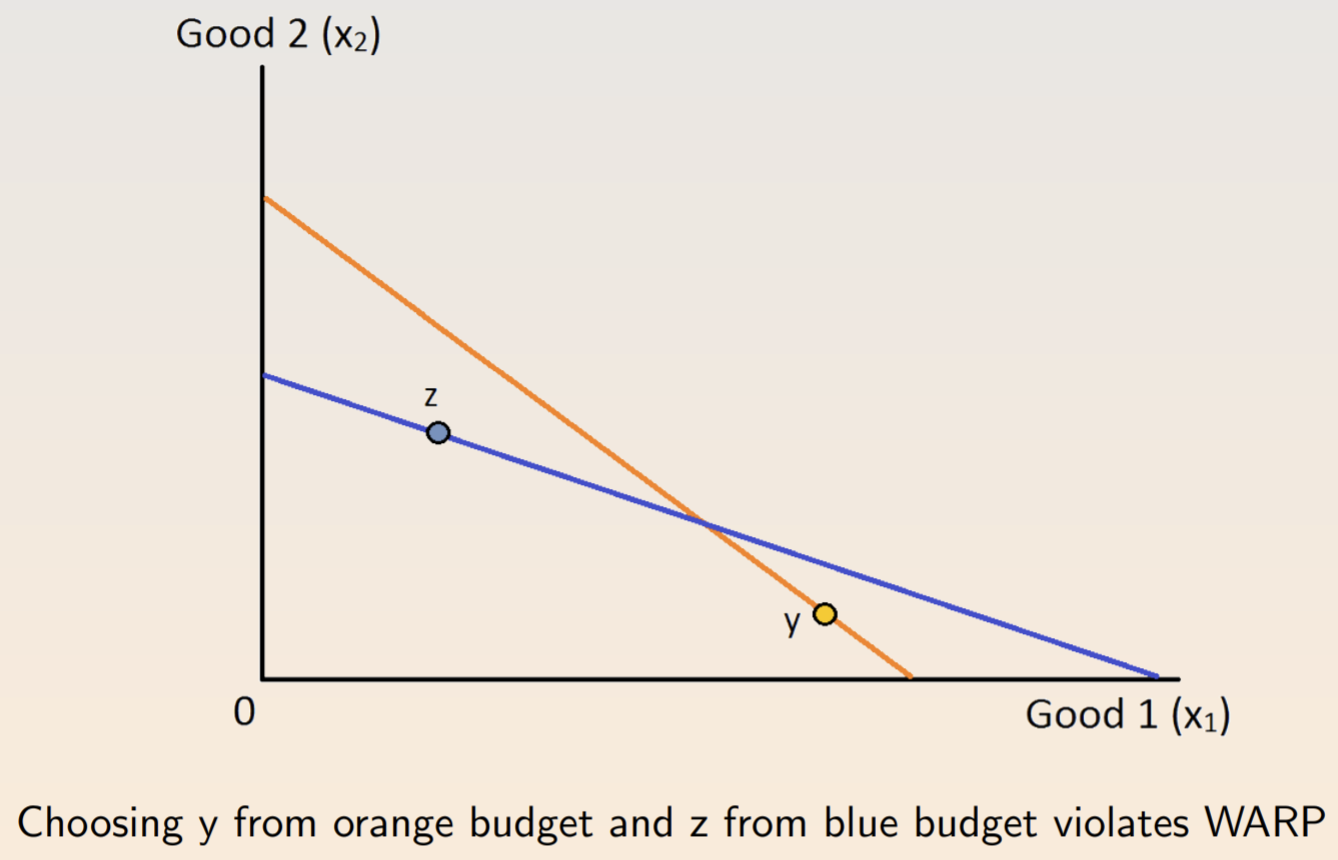
1. The weak axiom of revealed preference (WARP): If \(x\) is chosen when \(y\) is available, then there is no set of alternatives containing both \(x\) and \(y\) for which \(y\) is chosen but \(x\) is not.

Aggregating rational preference relations can lead to conundrums, including Condorcet’s paradox, where simple majority voting implies intransitive social preferences.

Endowment Effect

Standard theory equates willingness to pay and willingness to accept. It implies that indifference curves can be drawn without reference to current ownership. Thaler’s endowment effect describes situations where a person’s valuation of a good increases after they own it. It’s an example of loss aversion, causing losses to weigh heavier than gains. Some examples:

• Participants are given either a lottery ticket or $2. When given the opportunity, very few choose to switch, defying expectations.
• Median selling prices for pen and mug markets were more than twice the median buying prices.
• WTP for a 50% $10 lottery ticket was significantly lower than the WTA.
• Capuchin monkeys choose not to exchange for different foods.
• Winners of IPO lotteries choose to keep their stocks.

One way to measure WTP is the Becker-DeGroot-Marschak (BDM) method, where subjects will purchase an item if their self-stated WTP is higher than the listed price.

• An upset loss for LSU increased the length of Louisiana juvenile sentences by 35 days.

Status quo bias refers to a preference for the way things currently are. It could be caused by procrastination (where you put off a change) but it also could be habitual (if you’re used to making a decision).

• 401(k) procrastination is widespread and enrollment is much higher if it is automatic.

Framing Effects

The framing effect is when the presentation of a question affects responses. It’s closely related to reference points and crops up repeatedly.

• Narrow bracketing: breaking a complex decision into smaller parts without consideration for the whole. E.g. subjects prefer risky options in the context of losses even when transactions are equivalent.
• Mental accounting: separating household expenditures into buckets. E.g. a drink voucher induced greater spending on drinks.

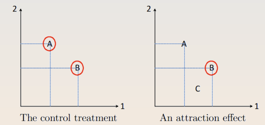
The attraction effect causes DMs to seek items that are asymmetrically dominated. In the treatment condition below, people are more likely to pick option B, which violates IIA and WARP.

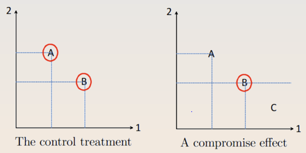
A related idea is the Overton window, where politicians will take extreme positions to make mildly extreme positions seem mild by comparison. The compromise effect induces people to pick options “in the middle.”

Satisficing

Substantive rationality attempts to further goals subject to constraints. Procedural rationality is the outcome of deliberation where outcomes are labeled as either “satisfactory” or “unsatisfactory” and the decision-maker stops at the first “good enough” option.

Assume a set \(A\) with \(M\) items where each option has a value from utility function \(U: X \to \mathcal{R}\). The subject has a probability distribution \(f\) capturing perceived values of each option. Each item has a cost of inspection \(k\). At any moment, the DM can stop inspecting items. After inspecting \(M-1\) items, we can stop and get \(\bar{u} - (M-1)k\) or continue and bet on the value \(u\) of the last item. The reservation stopping rule is to stop if the best thing so far is better than \(u^*\): \(k = \int^\infty_{u^*} (u-u^*) f(u) du\) The threshold \(u*\) is increasing in the cost of inspection, variance of \(f\), and mean of \(f\).

• Consumers purchase fewer goods when the post-tax price is visible. The effect is driven by dollar prices, which is why stores use .99 prices.
• The value of cars dips substantially when their odometers cross a 10k threshold.

Choice Overload

People can experience choice overload. In offers for loans, supermarket shelves, 401(k)s, and jam samples, people are more likely to buy if there are fewer choices. One explanation is the value of information, since fewer choices may imply a curation process. Another is cognitive overload, as it becomes harder to think through them all. In an experiment with many lottery choices, both effects seemed to be in play.

A related effect is flat rate bias, where customers prefer a simple cost structure. In a study of ISP customers, people irrationally preferred to pay a flat rate.

Models

One way to deal with violations of IIA is to see each DM as having a bag of preference relations so that each choice is maximal for one such bag. A related idea is to model multiple selves, including trying to influence your future self or versions of self with different levels of evidence.

Khaneman considers a fast-thinking System 1 and a slow thinking System 2. Real-world examples include self-control problems in a Congolese coupon program and procrastination among Amazon Mechanical Turk workers.

Time

Discounted Utility Model

Economist assume that utility is worth less when it’s received later rather than sooner. The standard discounted utility model assumes a consumer with a utility function \(u\), a discount factor \(\delta \in (0, 1)\), and outcomes \(x_0, ..., x_T\) at times \(t = 0, ..., T\). According to the net present value-style of discounting, her present utility is \(U(\{x_t\}^T_{t=0}) = \sum^T_{t=0} \delta^t u(x_t)\) This model is called stationarity or constant impatience. The DU model errs in a few ways:

1. The common difference effect: stationarity could be wrong, e.g. preference reversals
2. The absolute magnitude effect: large dollar amounts are discounted less than smaller amounts
3. Gain-loss asymmetry: losses are time discounted less than gains
4. Delay-speedup asymmetry: the willingness to accept a delay is 2-4x greater than willingness to pay for a speed up

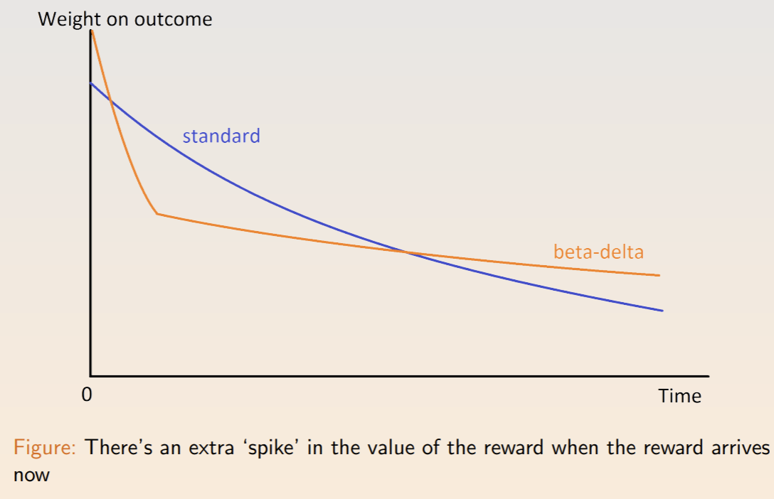
Time Inconsistency and Beta-Delta Model

Some preferences are time-inconsistent. For example, people will take $120 in seven months over $100 in six months, but also prefer $100 now over $120 in one month. These results face issues, since people could need money now, worry about the trouble of getting it later, or not believe that they’ll receive it at all.

We can capture time inconsistency with an extra parameter: \(U(\{x_t\}^T_{t=0}) = u(x_0) + \beta \sum^T_{t=1} \delta^t u(x_t)\) The difference between the two models is the extra premium on immediate rewards. This self-control problem can lead to different decision pathways.

Naivety

A naive DM doesn’t anticipate that their future selves will feel different. A sophisticated decision-making anticipates the problem and can build plans to resist the temptations. They can use commitment devices to ease the burden, like self-bans from casinos. Policies can also be designed to nudge people towards making correct decisions. One irregularity: people discount more when the time period is more finely partitioned.

Menu Choices and Temptation

We model temptations with menus. Suppose \(A\) is a menu of options and \(U(A, x)\) is the utility of picking \(x\). We can introduce the cost of self-control as \(s(A, x)\): \(U(A, x) = u(x) - s(A, x)\) The cost of self-control depends on the most tempting thing foregone: \(s(A, x) = \max_{y\in A} v(y) - v(x)\) The total utility of the menu is the utility of the ‘optimal’ item (temptation included): \(U(A) = \max_{x \in A} [u(x) + v(x)] - \max_{y \in A} v(y)\) People tend to prefer flexibility - the ability to choose from a menu later.

Another approach is to model willpower as a depletable resource with budget \(w\): \(U(A) = \max_{x \in A} u(x) \text{ subject to } \max_{y \in A} v(y) - v(x) \leq w\)

Scarcity and Agency

People subject to scarcity tend to have less patient. In experiments, ‘poor’ participants had self-control problems. When subjects have more agency over environmental stresses, they tend to have better self-control.

Other Anomalies

There are several behaviors beyond time inconsistencies that also contradict the exponential discounting model:

1. Preference for spread: People prefer rewards that are spaced out across time
2. Habit formation: consumption of a habit-forming good invests in a “habit stock,” pushing up the marginal utility of consumption
3. Rational addiction: drug users know that products are addictive but believe that gains outweigh future costs
4. Consumption constraints: people have inflexible expenditures like rent or mortgages, which is why people prefer consistent wages with sudden layoffs

Risk

Expected Utility Theory

The canonical model for uncertain outcomes is expected utility. Suppose a DM chooses among risky alternatives, where \(\mathcal{C}\) is the set of all \(n\) possible outcomes. A simple lottery has the form \(L = (p_1, ..., p_2)\) with \(p_n \geq 0 \forall n\) and \(\sum_n p_n = 1\). A compound lottery has outcomes that themselves are simple lotteries. A reduced lottery is a simple lottery that generates the simple distribution for some compound lottery.

We assume consequentialism, that only the reduced lottery over final outcomes matters. The set \(\mathcal{L}\) denotes all the simple lotteries over outcomes \(\mathcal{C}\), over which DM has a rational preference relation \(\succsim\).

Continuity requires that small changes in probabilities don’t alter the DM’s ordering between two lotteries. IT guarantees the existence of a utility function for \(\succsim\). Independence guarantees the independence axiom for all \(L_1, L_2, L_3\) and \(p\): \(L_1 \succsim L_2 \text{ iff } pL_1 + (1-p)L_3 \succsim pL_2 + (1-p)L_3\) A utility function \(U : \mathcal{L} \to \mathbb{R}\) has a von Neumann-Morgenstern expected utility function if there is an assignment to the \(N\) outcomes where for every simple lottery $L$ we have: \(U(L) = u_1p_1 + ... + u_Np_N\) EU is cardinal - the magnitude matters. A rational preference relation \(\succsim\) has an expected utility form if it satisfies the continuity and independence axiom.

Paradoxes

Consider the Allais paradox. People will choose a riskier option when the difference in probability is smaller. We could relax the independent axiom or introduce non-consequentialist preferences.

Also consider the Ellsberg paradox. People experience ambiguity aversion: they prefer known probabilities over unknown probabilities.

In Machina’s paradox, people would prefer an inferior option (“stay at home”) when the alternative (“movie about Venice”) is paired with a disappointment-inducing main option (“trip to Venice”).

Worst of all, when outcomes are frame as losses, people seem to be risk-seeking.

To deal with the St. Petersburg paradox, we can introduce a vNM utility function over each distribution function \(F\): \(U(F) = \int u(x) dF(x)\) Here, \(u(\cdot)\) is the Bernoulli utility function. A DM exhibits risk aversion if the degeernate lottery yielding \(\int x dF(x)\) is at least as good as \(F(\cdot)\). Equivalently, DM has a concave utility function and requires a risk premium. We can measure risk aversion with the Arrow-Pratt coefficient of absolute risk aversion: \(r_A(x) = - \frac{u''(x)}{u'(x)}\) For percentage gains and losses, the coefficient of relative risk aversion is: \(r_R(x) = - \frac{xu''(x)}{u'(x)}\) Nonincreasing relative risk aversion means that an individual becomes more risk seeking as their wealth increases. The constant absolute risk aversion (CARA) utility function is: \(u(x) = -e^{-\alpha x}, r_A(x) = - \frac{-\alpha^2e^{-\alpha x}}{\alpha e^{-\alpha x}} = \alpha\) The **constant relative risk aversion ** (CRRA) utility function is: \(u'(x) = \frac{x^{-\rho}}{1-\rho}, r_A(x) = -\frac{xu''(x)}{u'(x)} = \rho\) We could measure the riskiness of a gamble by finding the reciprocal of the absolute risk aversion of the CARA utility function that makes the DM indifferent.

Consider two random variables \(x\) and \(y\) with cdfs \(F\) and \(G\). F first order stochastically dominates G if every EU maximizer with monotone preferences prefers F to G, i.e. \(F(\eta) \leq G(\eta) \forall \eta\). F second order stochastically dominates G if every risk-averse DM prefers F to G, i.e. \(\int^\eta_a G(x) dx \geq \int^n_a F(x)dx \forall \eta \geq 0\).

Rabin and Thaler show that if people reject a 50-50 gamble between winning $11 and losing $10, then they ought to reject the same gamble between losing $100 and winning infinite money. These are inconsistent with a model where the DM considers lifetime wealth.

A DM risk averse agent has incentives to purchase insurance at a rate greater than expected losses. Suppose a DM has initial wealth \(W\) and faces a loss of \(L\) with probability \(p\). Insurance pays \(\$q\) in event of a loss and the premium per dollar of coverage is \(\pi\). The utility maximization problem is: \(\max_q EU = pu(W-L - \pi q + q) + (1-p)u(W - \pi q)\) Taking the derivative: \(pu'(W - L + q^*(1-\pi))(1- \pi) - (1-p)u'(W - \pi q^*)u'(W - \pi q^*)\pi = 0 \\ \implies \frac{u'(W - L + q^*(1 - \pi))}{u'(W- \pi q^*)} = \frac{1-p}{p} \frac{\pi}{1-\pi}\) The firm’s expected profit is \((1-p)\pi q - p(\pi q - q)\) which, under zero profit, implies \(\pi = p\), an actuarially fair premium. Substituting back, \(q^* = L\) - the consumer insures all losses.

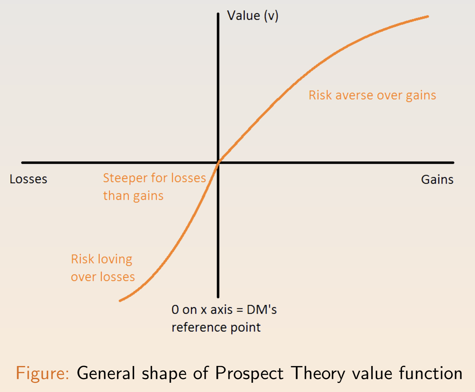
The certainty effect is a premium for guarantees (either probability 1 or 0). The reflection effect is the tendency to display risk aversion for positive prospects and risk seeking for negative prospects. The isolation effect is the tendency to look only at the amount when the probabilities are small and similar.

Prospect Theory suggests that people use an editing phase to simplify choices before making a decision. People assign a perceived probability \(\pi(p)\) and a subjective value \(v(x)\). A prospect \((x, p; y, q)\) involves up to two non-zero outcomes \(x, y\) with probabilities \(p, q\) and nothing with probability \(1-p-q\). The total value is: \(V(x, p; y, q) = \pi(p)v(x) + \pi(q)v(y)\) The value function incorporates the reflection effect and loss aversion:

The decision weight function reflects the certainty effect and isolation effect:

Empirical results suggests the weight function is concave up to \(p=0.4\) and convex afterwards. One model is a two-parameter function comprising discriminability (diminishing sensitivity to changes away from endpoints) and attractiveness (difference in baseline attractiveness).

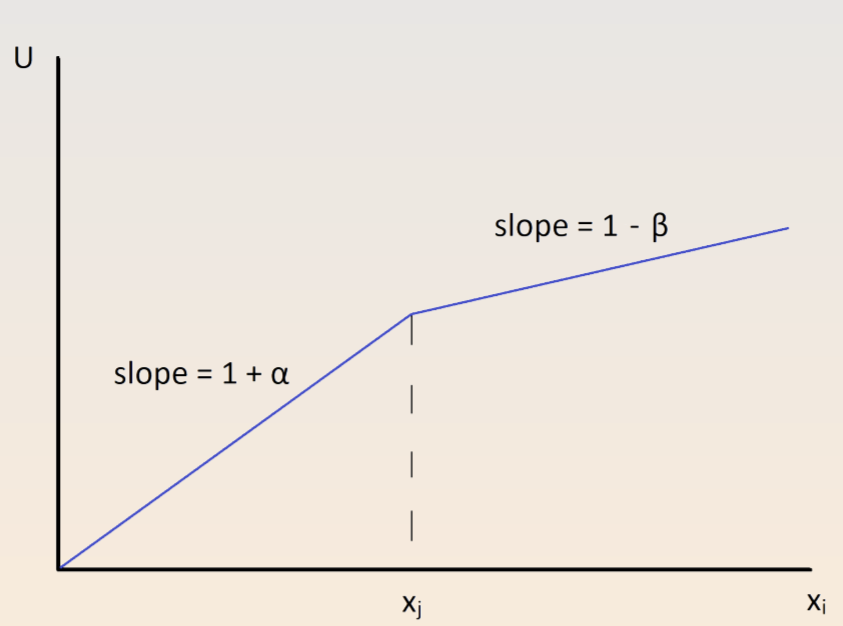
To account for loss aversion, we can consider a reference point \((r_1, r_2)\) for each bundle \((x_1, x_2)\). The new utility depends on the reference point: \(u_i (x_1 - r_i) \text{ if } x_i > r_1\\ -\lambda u_i(r_i - x_i) \text{ if } x_i < r_i\) The WTP is less than the WTA for \(\lambda > 1\). In experiments, the correlation between \(\lambda\) and the WTP/WTA gap is 0.63. Phenomena consistent with loss aversion include the equity premium puzzle, labor supply, and disposition effect.

One consistent result is information aversion. For a two sequential 50-50 gambles of +200 or -100, the utility depends on whether the DM knows the intermediate result. This manifests as the ostrich effect, where investors log in to their accounts less when stocks are down.

Reference dependency can affect effect. Define effort as \(e\) with cost \(c(e)\), reference point \(r\), and relative weight on reference point \(\eta\). Above and below the reference point the individual maximizes: \(\max_e e + \eta (e-r) - c(e) \text{ for } e \geq r\\ \max_e e + \eta \lambda (e - r) - c(e) \text{ for } e < r\) The optimal choice balances the marginal benefit and cost of effort: \(1 + \eta = c'(e^*) \text{ for } e \geq r\\ 1 + \eta \lambda = c'(e^*) \text{ for } e < r\) Subjective expected utility (SUE) accounts for uncertainty. SEU associates each state with a probability, each prize with a utility, and choose the act with the highest EU. Letting \(X\) denote the set of prizes, \(\Omega\) a finite set of states, and \(F\) the resulting set of acts, a preference relation \(\succsim\) has a SEU if there exists a utility function where \(f \succsim g\) if and only if: \(\sum_{w \in \Omega} \pi(\omega) u(f(\omega)) \geq \sum_{w \in \Omega} \pi(\omega) u(g(\omega))\) Rank dependent utility (RDU) models probability weight of a prize based on the probability of its arrival and the relative rank of the prize. The weight of the top prize is the decision weight of its probability, while the weight on the \(n\)th best is the weight on probability of getting something at least as good minus the probability of getting something better than it. RDU helps us explain Allais paradox.

Maxmin expected utility (MEU) suggests a DM maximizes the minimum utility across different probability distributions. It helps to explain the Ellsberg paradox and no-trade region prices. Formally, using the previous setup and a convex set of probability functions \(\Pi\), a MEU representation exists for a preference relation \(\succsim\) if \(f \succsim g\) if and only if: \(\min_{\pi in \Pi} \sum_{w \in \Omega} \pi(\omega)u(f(\omega)) \geq \min_{\pi \in \Pi} \sum_{w \in \Omega} \pi(\omega) u(g(\omega))\)

Games

Games and Strategies

A game consists of

• players: a list of all relevant players
• moves: what each player can do
• information: what each player knows
• payoffs: vNM utilities as a function of every player’s actions

The objects of interest are

• strategy: a contingent plan of action for each player
• strategy profile: a collection of strategies for each player
• solution concept: a strategy profile that is likely

We assume complete information by default. The normal form (or strategic form) of a game involves

• a set of players: \(N\)
• the pure-strategy space: \(S_i\)
• a payoff function for each player \(i\) where \(u_i : S_1 \times ... \times S_n \to \mathbb{R}\)

Payoffs represent the players’ preferences, but aren’t necessary monetary. Models are underdetermined - if one hypothesis is consistent, an infinite number are.

We represent a finite two-player game with two moves as a matrix. In the example below, the “row” player has strategies \(T\) and \(B\), while the “column” player has strategies \(L\) and \(R\). The numbers represent the payoffs of player 1 and player 2.

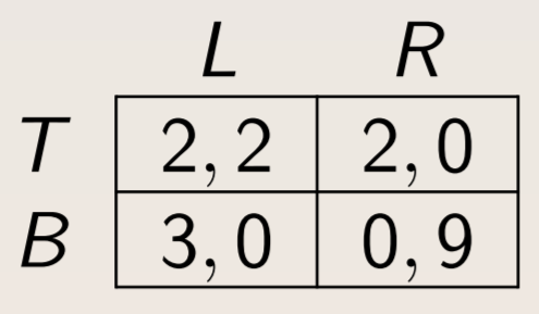
A pure strategy involves taking actions for sure. A mixed strategy is a probability distribution over pure strategies. A strategy for \(i\) is the best response if there exist no other strategy that yields a higher expected payoff.

Dominance and Equilibrium

A Nash equilibrium is a strategy profile where every player’s strategy is a best response to the strategies played by the other players. A strategy for player \(i\) is strictly dominated if there’s another strategy with a greater payoff for all the strategy profiles of the other player(s). A strategy is weakly dominated if another strategy yields a payoff at least as high for all strategy profiles of the other players and a greater payoff for at least one.

Mixed Strategies and Reaction Functions

Nash equilibria are tricky. Suppose there is a \((1, 1)\) payoff in a two-player two-move game only if they both choose the same move, and \((0, 0)\) otherwise. In addition to the \((A, A)\) and \((B, B)\) cases, another equilibrium is a mixed strategy with equal probabilities for both. In general, each player has a mixed strategy that renders the other player indifferent, and if they simultaneously do so, they reach equilibrium.

A reaction function graphs each player’s best response as a function of the probability the other play puts on one of the actions. Visually, the intersections are Nash equilibria.

Level k Reasoning

A minimax strategy minimizes the maximum payoff of the opponent. In rock-paper-scissors, the optimal strategy is uniformly randomness. In practice, soccer players perform kickoffs consistently with minimax.

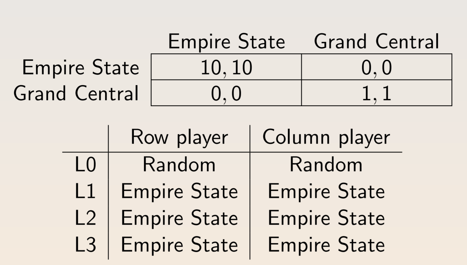
One way to model a player’s thought process is level-k reasoning:

• L0: an ‘unsophisticated’ player who chooses based on some heuristic
• L1: a strategy based on an opponent’s L0 behavior
• L2: a strategy based on an opponent’s L1 behavior
• and so on..

It’s most useful in modeling behavior in novel situations. A similar approach is to have level k players act based on distributions of lower types.

In beauty context, everyone writes down an integer between 0 and 100. The player with the number closest to 2/3rds of the average wins. The higher the level of a player, the lower the number they will guess. Some responses:

1. Fixed point - zero is the unique equilibrium
2. Iterated deletion - a rational player never chooses greater than 66; others will know this and never choose greater than 44; so on to 0
3. Iterated best reply - all players think they’re one level deeper
4. Iterated best reply II - players can think that other players are on more than one level

In real world experiments, players display behavior from each of these categories, with most people using level-k reasoning. Cognitive hierarchy involves a distribution of step \(k\) players assumed to be Poisson, where \(\lambda = 1.61\). Experimental results aren’t perfect because a categorization could be spurious.

Consider the 11-20 money request game. Each player can choose a number of dollars to receive between 11 and 20; they receive a $20 bonus if they ask for one dollar less than the other person. Most people displayed L1, L2, and L3 reasoning. Increasing the salience of $20 increases the rate of L1 reasoning.

Subjects are often better at coordinating than the mixed-strategy result. K-level reasoning explains why subjects can outperform the mixed-strategy Nash equilibrium.

In hide and seek, hiders must use k-level reasoning to predict which boxes seekers will view as salient. Subjects tend to see endpoints and distinctly labeled boxes as salient, leading both hiders and seekers to avoid those boxes.

In experiments, cognitive ability seems to be positively correlated with level. Agreeable and emotionally stable subjects also had higher levels.

Backward Induction

Backwards induction is about using expect future behave to induce present behavior. The extensive form of a game uses a game tree to represent the order of a game.

A decision node is a point where a player makes a move. The initial decision node is the first point. Each branch represents a choice, and the game ends at a terminal node. An information set links decision nodes so that a player only knows that a node in the information set has been reached. A strategy is sequentially rational if it is optimal at every point in the game tree. Every finite game with perfect information has a pure strategy Nash equilibrium that can be derived through backwards induction. At any given point of induction, the set of Nash equilibria that survive is called the set of Subgame Perfect Nash Equilibria.

Key point: a strategy is a contingent plan of action, which means strategies must be completely specified.

A subgame is a subset of game which begins at an information set containing a single decision node, contains only the successors, and recursively includes information sets. A strategy profile is a subgame perfect Nash equilibrium of a game if it induces a Nash equilibrium in every subgame.

The centipede and race to 100 games both test backward induction skills. Skilled chess players seem to perform better at backward induction.

Repeated Games

In the Chainstore paradox, backward induction implies that a store never has a logical reason to fight an entrant, even to deter future entry. In this sense, the result of SPNE is unconvincing. When the repeated game has multiple Nash equilibria, SPNE is less restrictive.

The grim strategy involves cooperating initially, and then defecting indefinitely whenever the other player first defects. In the infinitely repeated Prisoner’s Dilemma, the grim strategy is mutually preferable for high enough discount rate. This model predicts that firms will collude to set high prices if they are sufficiently patient.

The Folk Theorem states that for any feasible pair of individually rational payoffs \((\pi_1, \pi_2) >> (\not\pi_1, \not\pi_2)\), there exists a \(\delta\) such that \((\pi_1, \pi_2)\) are the average payoffs in SPNE. In experiments, subjects are more likely to cooperate if a game is more likely to continue. Across a longer time span, players may also bet on the chance that the other subject is a “grim” player.

Fairness

Games

The main games we will examine are the ultimatum/dictator games, public goods contribution games, and trust games.

In the ultimatum game, player 1 proposes a division of $10 and player 2 can either accept or reject the division. In the dictator game, player 2 has no such discretion. In both games, subjects chose to make large, fair offers between 40% and 50%. In experiments, men split more when there is a face which may be because men are less socially aware by default.

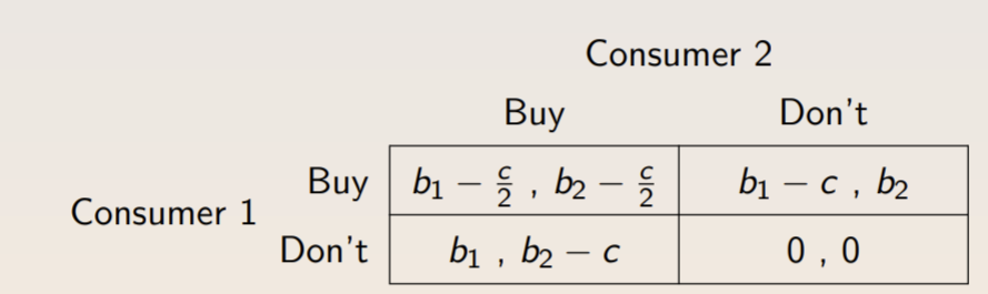
In public goods games, people contribute in the hopes of conditional cooperation. The table below displays the incentives for free-riding - if consumers \(1, 2\) split the cost of a public good from which they receive benefit \(b_i\), they each have incentives to not contribute if \(b_i < c\).

In an experiment, subjects that were paid by earning ranking or who simply knew of their rank quickly reduced their contribution to the public good. Across multiple rounds, cooperation decreases among both partners and strangers, suggesting that subjects care about future periods.

In trust games with payback, trust was not reciprocated in over half of cases, yet subjects who knew this still sent money. When individuals are sorted and paired by trustworthiness, they become more cooperative over time. Women seem to return more. Seeing a picture induces more trusting, and senders will pay to see a picture. In simulations of labor markets, a higher wage or thoughtful gift is reciprocated with more work.

Fairness and Norms

People have a preferences for redistribution. The motives come primarily from self-interest and secondarily from income uncertainty; WTP is 0.4% of ones own payoff for a 10% decrease in inequality. Attitudes about social welfare can be easily induced with cues.

Queues are seen as the most fair way to allocate tickets, followed by a lottery and then by an auction. People think raising prices is more fair than opportunistically lowering wages. We tend to weigh actual losses greater than opportunity costs. Removing a discount is seen as much more fair than a price hike.

In games, people will use reputations or punishments to enforce social norm. The Fehr-Schmidt utility function models inequality aversion as follows, where \(\alpha\) is the amount that \(i\) suffers from disadvantageous inequality and \(\Beta_i\) is the amount that \(i\) suffers from advantageous inequality.

Since \(\Beta_i\) is constrained to be less than 1, players will always accept advantageous offers. For higher \(\alpha\), players are more stringent about equality. Other models are based on ERC (equity, reciprocity and competition) and the total/lowest payoffs.

Incentives and Crowding Out

In some settings, cash incentives can crowd out intrinsic motivation to do the right thing. In others, they can crowd in intrinsic incentives. A famous example of a daycare found that charging a fine for lateness increased the number of late-coming parents, with an effect persisting after the fine was lifted. A similar result was found for building a nuclear waste repository.

Two explanations are self-determination (substitution of motivators) and self-esteem (their intrinsic motivation isn’t being recognized). If external interventions are controlling rather than supporting, then self-determination and self-esteem are impaired.

We can model social norm with a modified utility function: \(U = u(c) - \gamma (x - \bar{x})^2\) Notice that losses from deviations are symmetric and increase non-linearly. When researchers measured and modeled social acceptability in the dictator and bully games, the models matched the data very well.

Prosocial incentives seem to be less effective than selfish incentives, mandatory prosocial incentives even less so. In the field, pay-what-you-want models with proportional donations to charities elicit the most payment.

Beliefs

Statistics

Beliefs are important for behavior, and beliefs update with new information. Bayes’ Theorem models the mathematically correct way to update events: \(Pr(A|B) = \frac{Pr(B|A)Pr(A)}{Pr(B)}\) People are bad at applying Bayesian reasoning.

Biases Galore

They also are bad at randomizing, with a bias towards the number 7 and the color blue. People suffer from the gambler’s fallacy (after three heads in a row, the chance of another is <50%) and the law of small numbers (introducing extra switches in random sequences). Even asylum judges, loan officers, and MLB umpires suffer from these biases. In contrast, the hot hand fallacy causes people to think that random processes enter a “hot” state, especially in sports.

People are insensitive to sample size, failing to understand the law of large numbers. Subjects also suffer from correlation neglect, failing to detect and use correlating information. Simultaneously, people are overconfident in precision and ability, giving overly narrow confidence intervals. Men seem to be more overconfident, on average.

People experience motivated beliefs as a source of optimism or social signaling. They use selective memory, conservative updating of beliefs, asymmetric updating, and information avoidance to improve their self-image or maintain beliefs. In experiments, subjects ignore negative feedback later on, but will consider it with high enough incentives.

Alerting a DM to the expectation of donating causes them to avoid the ask. Similarly, telling them that lying is widespread causes them to lie more.

The conjunction effect is a bias in which people substitute a question about likelihood for a question about representativeness. One explanation is poor wording, but even raising the stakes and picking informed audiences doesn’t erase the effect.

People are bad at portioning probability - especially when asked to consider small portions, they drastically overestimate probabilities. They suffer from projection bias, with shoppers overestimating their hunger. They also suffer diversification bias, preferring a variety only when planning ahead. A model of projection bias for a future state \(s\) is \(\hat{u}(c, s) = (1-\alpha)u(c, s) + \alpha u(c, s')\) where \(\alpha\) is a measure of projection bias and \(s'\) is the current state.

Persuasion

The persuasion rate for a behavioral outcome can be expressed as \(f = 100 \times \frac{y_T - y_C}{e_T - e_C} \frac{1}{1-y_0}\) where:

• \(T\) and \(C\) refer to the treatment and control groups, respectively.
• \(e_i\) is the share of group \(i\) that receives the message.
• \(y_i\) is the share of group \(i\) that adopts the behavior
• \(y_0\) is the share that would adopt without the message, usually approximated as \(y_c\) when unknown

Persuasion can be mediated by beliefs (with updating), preferences (advertising affect utility), and information (costs of acquiring info and paying attention).

Dialectic Model

The DM makes a best guess about the state of the world. They maintain two frames with means \(\mu_L, \mu_H\) and widths \(w_L, w_H\). The DM’s belief is the weighed average of the two: \(\hat{u} = \frac{w_H^s}{w_L^2 + w_H^s} \mu_L + \frac{w_L^2}{w_L^s + w_H^2} \mu_H\) where \(s\) tracks the level of skepticism. A skeptical DM punishes width but people vary, which explains why politically, conservatives may adopt the strategy of extreme beliefs, appealing to credulous DMs. People also don’t react to more of existing evidence.

Information Cascades

People close ot each other display conformity. Suppose a new behavior has an adaption cost of \(\frac{1}{2}\) and a value \(v\), either 0 or 1 with equal probability. Suppose that each individual has a private signal that is correct with \(p > \frac{1}{2}\). If one person reacts to their private signal, a second person updates their beliefs to be in conformity. Because of these cascades, people can ignore their private signals.

In lab experiments, people quickly form cascades. In terms of incentives, majority rule institutions had the fewest information cascades, followed by individualistic institutions and conformity-rewarding institutions. One form of spillover is awareness: even bad reviews of unknown authors increase sales.