
Notes: ECON 101A / Microeconomics
Published:
These notes are for the Spring 2021 version of Economics 101A: Microeconomic Theory. I did not go to lecture, so these may not reflect the content on the test. The notes are based on the 12th edition of Microeconomic Theory by Nicholson and Snyder.
Midterm 1
Economics
The ceteris paribus assumption restricts the forces at play. In economics, controlled experiments are usually impossible to conduct, so statistical methods are used to control for other factors.
Factors that are outside of a decisionmaker’s control, such as prices, are called exogenous variables. Factors within their control, such as quantity bought, are called endogenous variables. Often, we want to study the effect of changing an exogenous variable.
Economic actors are assumed to be optimizers. It helps to create solvable models and the assumption has some empirical validity.
Economists disagree over the positive-normative distinction. Some economists believe in pure positive analysis, where economics should only describe events. Others believe that economics is inevitably laden with views on ethics, morality, and fairness.
Originally, economists like Adam Smith struggled with the water-diamond paradox. Water, imminently useful, was cheap. Diamonds, which had little practical use, were expensive. The marginal revolution resolved this paradox. Prices reflect the marginal evaluations of demanders and producers. Water is cheap because it has little marginal value and a low cost of production. Diamonds are expensive because they have high marginal value and a high cost of production.
The production possibility frontier is models tradeoffs between two goods. Because of scarcity, producing good A imposes an opportunity cost in terms of good B.
Modern developments include mathematical foundations sophisticated models of markets, incorporation of uncertainty and information, and the study of behavioral economics. Computers now enable researchers to leverage large amounts of real world data to test models.
Optimization
To maximize a function \(f\), we must have \(f'(x^*) = 0\) and \(f''(x^*) < 0\).
Elasticity between two goods \(x\) and \(y\) is defined as \(e_{y, x} = \frac{\frac{\delta y}{y}}{\frac{\delta x}{x}} = \frac{dy(x)}{dx} \frac{x}{y}\).
Implicit functions reveal tradeoffs between variables. For example, suppose we have \(f(x_1, x_2) = 0\). We can express \(x_2\) in terms of \(x_1\) so that \(x_2 = g(x_1)\). Differentiating with respect to \(x_1\) yields \(\frac{dg(x_1)}{dx_1} = -\frac{f_1}{f_2}\).
Comparative statics denotes the effect of an exogenous variable \(a\) on an endogenous variable \(x\). In other words, \(\frac{dx(a)}{da} = - \frac{\frac{df}{da}}{\frac{df}{dx}}\).
To maximize a function of multiple variables, the partials with respect to each variable must equal 0 and the second partials must be negative.
To assess the impact of an exogenous variable \(a\) on \(y(x)\), we could solve for \(x^*\) in terms of \(a\) and compute \(y(x^*)\). However, we could also apply the Envelope Theorem and immediately conclude that \(\frac{dy^*}{da} = x^*(a)\). The theorem also holds for the many variable case, so that \(\frac{dy^*}{da} = \frac{df}{da}\|_{x_i = x_i^*(a)}\).
Langrange multipliers are used for constrained optimization. To maximize \(y=f(x_1, x_2,..., x_n)\) subject to constraint \(g(x_1, x_2, ..., x_n) = 0\), set up the Langrangian \(\mathcal{L} = f + \lambda g\). The conditions are \(\frac{\delta \mathcal{L}}{\delta x_i} = f_i + \lambda g_i = 0\) for each good $x_i$ and \(g = 0\).
The multiplier can be interpreted as the benefit-cost ratio, i.e. \(\lambda = \frac{mb}{mc}\) for all \(x_i\). It means that if the constraint were slightly relaxed, it wouldn’t matter which \(x_i\) were increased.
The envelope theorem means \(\frac{dy^*}{da} = \frac{d \mathcal{L}}{da} (x_1^*,...,x_n^*; a)\).
Often, we wish to deploy inequality constraints such a \(g(x_1, x_2) \geq 0\) or \(x_1 \geq 0\). We can use slack variables, such as \(g(x_1, x_2) - a^2 = 0\) and \(x_1 - b^2 = 0\). Substituting, we introduce the additional first-order conditions \(\frac{d\mathcal{L}}{da} = -2a\lambda_1\) and \(\frac{d\mathcal{L}}{d\lambda_1} =g(x_1, x_2) - a^2 = 0\).
Preferences
Preference relations have three properties. First, completeness. For two options A and B, it must be the case that either A is preferred to B, B is preferred to A, or that they are equally attractive. Second is transitivity. If A is preferred to B and B is preferred to C, then A is preferred to C. Third is continuity. If A is preferred to B, then options “close enough” to A are also preferred to B.
Utility is only defined as a monotonic transformation. We can’t ask “how much more is A preferred to B?” because there isn’t a unique answer. One consequence is that utility can’t be compared across individuals. Ceteris paribus is in effect: when utility is specified as a function of goods, then it is assumed that all other factors are held constant. A utility function of goods takes the form:
\[U(x_1, x_2, ..., x_n)\]Indifference curves represent all of the combinations of goods with a given utility \(U_1\). The slope of the indifference curves indicates the trade someone is willing to make between goods. Indifference curves never intersect. Otherwise, the axioms of transitivity suggest produce a contradiction.
Goods face diminishing marginal utility, since people do not want too much of any one good. A diminishing MRS produces a convex indifferent curve.
There are several key utility functions. One common function is Cobb-Douglas, where \(U(x, y) = x^\alpha y^\beta\), often normalized to \(U(x, y) = x^\alpha y^{1-\alpha}\).
Linear indifference curves are generated by \(U(x, y) = \alpha x + \beta y\). These denote perfect substitutes, since MRS is constant. An example would be indifference towards where to buy gasoline.
Perfect complements denote pairs of goods that “go together,” like coffee and cream. In the extreme case, \(U(x, y) = \min (\alpha x, \beta y)\). The ratio of goods consumed is given by \(\frac{y}{x} = \frac{\alpha}{\beta}\).
The Constant Elasticity of Substitution (CES) function takes the form of \(U(x, y) = [x^\alpha + y^\alpha]^{\frac{1}{\alpha}}\), and it incorporates each of the previous utility functions. As \(\alpha \to 0\), it approaches Cobb-Douglas. As \(\alpha \to -\infty\), it approach perfect complements.
When the utility function takes in many goods, the MRS between two goods is
\[MRS = -\frac{dx_2}{dx_1}|_{U(x_1 x_2, ..., x_n) = k} = \frac{U_{x_1}(x_1, x_2,..., x_n)}{U_{x_2}(x_1, x_2, ..., x_n)}\]Budget Constraints
If someone faces a budget constraint \(p_xx+p_yy \leq I\), then their possible combinations of goods is bounded by a triangle with slope \(-\frac{p_x}{p_y}\). The first order conditions is that the slope of the indifference curves equals the slope of the indifference curve, i.e. that:
\[\frac{-p_x}{p_y} = \frac{dy}{dx}|_{U = constant}\]Tangency is only a sufficient condition when the MRS is diminishing, which guarantees that the utility function is quasi-concave. Often, there can be a corner solution, e.g. \(x = x^*\) and \(y = 0\), which we must check separately.
In the \(n\) good case, we have \(\mathcal{L} = U(x_1, x_2,..., x_n) + \lambda(I - p_1x_1 - p_2x_2 - ... -p_nx_n)\). The first order conditions dictate that \(MRS(x_i for x_j) = \frac{dU/dx_i}{dU/dx_j} \frac{p_i}{p_j}\). Here, \(\lambda\) represents the marginal utility per extra dollar of income, which is constant across goods.
To account for corner solutions, we consider the case where \(\frac{d\mathcal{L}}{dx_i} = \frac{dU}{dx_i} - \lambda p_i \leq 0\), where if the the marginal utility is less than the basket-wide marginal utility per income, then none of that good is consumed, i.e. \(x_i = 0\).
Since demand functions dictate the consumption of goods such that \(x^* = x(p_1, p_2, ..., p_n, I)\), utility can be rewritten as a function of exogenous variables such that \(U = V(p_1, p_2, ..., p_n, I)\). Indirect utility allows us to assess the effect of a tax on one good. The lump sum principle states that for the same amount of revenue, an income tax will depress utility less than a tax imposed on one good.
Expenditures minimization involves an expenditure function \(E = p_1x_1 + p_2x_2 +...+p_nx_n\) with constraint \(\bar{U} = U(x_1, x_2, ..., x_n)\). Utility maximization with a budget constraint and expenditure minimization with a target utility constraint are equivalent problems. Notice that this is the inverse of the utility function. In practice, the expenditure function is more useful because the envelope theorem helps reveal key elements of demand.
Expenditure functions share several properties. First, homogeneity. A doubling of all prices will double the required expenditure. Second, expenditure functions are nondecreasing in prices. That is to say, \(\frac{dE}{dp_i} \geq 0\) for all goods. Third, expenditure functions are concave in prices. If the price of a good decreases, expenditure decreases even faster because it can efficient reallocate goods.
Demand
A demand function for a good \(x_i\) takes the form \(x_i ^* = x(p_{x_1}, p_{x_2}, ..., I)\). One property is homogeneity: \(x_i^* = x_i(tp_1, tp_2, ..., tp_n, tI)\). Changing all prices and incomes with the same proportion will not change quantity of goods demanded.
Consumption of normal goods increases and income increases. For inferior goods, quantity purchased decreases as income rises. If there are only two goods, if one good is inferior then the other must be normal.
When a good’s price changes, there are two forces at play that affect consumption of that good. First, there is the substitution effect, as the MRS changes to reflect the new ratio of prices. Second, there is the income effect, as a decrease in price increases real income.
For normal goods, these effects reinforce each other. For inferior goods, the substitution effect still increases consumption, but the increase in income works in the opposite direction. When the income effect is strong enough, an increase in the price of an inferior good can paradoxically increase consumption.
Utility varies along an uncompensated demand curve \(x = x(p_x, p_y, I)\), since income and other prices are constant. A decline in \(p_x\) therefore increases purchasing power. We could also hold real income constant, forming a Hicksian or compensated demand curve \(x^c = x^c(p_x, p_y, U)\). Notice that the Hicksian of a good \(x\) can be obtained by differentiating the expenditure function with respect to \(p_x\). The compensated demand curve must have a negative slope: an increase in price will always decrease the amount consumed. Because the income effect doesn’t play a role for compensated demand curves, the uncompensated curve is more price-sensitive.
Now, notice that \(x^c(p_x, p_y, U) = x[p_x, p_y, E(p_x, p_y, U)]\). By differentiating with respect to \(x\), we obtain
\[\frac{dx^c}{dp_x} = \frac{dx}{dp_x} + \frac{dx}{dE} * \frac{dE}{dp_x}\]and rearrange to yield
\[\frac{dx}{dp_x} = \frac{dx^c}{dp_x} - \frac{dx}{dE}*x^c\]We can interpret this to mean that the change in quantity consumed to price is equal to the compensated change in consumption (the substitution effect) minus the sensitivity of consumption to expenditure multiplied by the sensitivity of expenditure to a change in a good’s price (the income effect). The consequence is that we can decompose a good’s price sensitive into the income effect and substitution effect.
Midterm 2
Altruism
Utility maximization can account for altruism. Suppose that Kevin and I have utility function \(u(c)\) with \(u'>0, u''<0\). If I am altruistic towards Kevin and donate \(D\), I maximize \(u(c_P) + \alpha u(c_K)\) with \(\alpha > 0\) subject to \(c_P \leq M_P - D\), while Kevin selfishly maximize \(u(c_K)\) subject to \(c_K \leq M_K + D\).
Substituting, we can derive \(\max u(M_P - D) + \alpha u(M_K + D)\) with FOC \(-u'(M_P - D^*) + \alpha u'(M_K + D^*)\) and SOC \(u''(M_P - D^*) + \alpha u''(M_K + D^*) < 0\).
If \(\alpha = 1\), then \(u'(M_P - D^*) = u'(M_K + D^*)\) so \(D* = \frac{M_P - M_K}{2}\)—if Kevin earns less than me, then I donate such that the incomes equate.
We can compute comparative statics to altruism, donor income, and recipient income: \(\frac{\delta D^*}{\delta \alpha} = - \frac{u'(M_K + D^*)}{u''(M_P - D^*) + \alpha u''(M_K + D^*)} > 0\\ \frac{\delta D^*}{\delta M_P} = - \frac{-u''(M_P - D^*)}{u''(M_P - D^*) + \alpha u''(M_K + D^*)} > 0\\ \frac{\delta D^*}{\delta M_K} = - \frac{\alpha u''(M_K + D^*)}{u''(M_P - D^*) + \alpha u''(M_K + D^*)} < 0\)
Risk Aversion
For risk averse people, extra resources may provide decreasing marginal utility. Someone who makes $50,000 a year would be unlikely to accept a $20,000 bet on a coin flip because the negative utility of a $30,000 income is worse than the additional utility of a $70,000 income. You can see this graphically below for a starting income of \(W_0\) and earnings of \(h\). The certainty equivalent, \(CE_A\), is the amount that people would be willing to pay to avoid taking the bet.
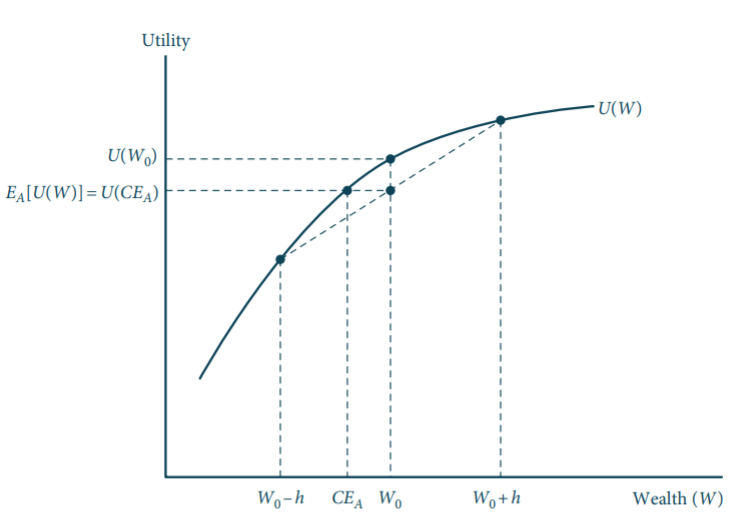
We can measure absolute risk aversion with Pratt’s risk aversion measure \(r(W) = -\frac{U''(W)}{U'(W)}\). The amount a risk-averse individual is willing to pay is proportional to Pratt’s measure so that \(p = kr(W)\) where \(k = E(h^2)/2\) and \(h\) is a random variable representing winnings.
However, it often makes more sense to ask of relative risk aversion, since an increase in wealth may reduce absolute risk aversion. If we assume wealth is inversely related to risk aversion, then \(rr(W) = Wr(W)\) is constant.
Risk averse people are willing to purchase unfair insurance to cover losses. We can model \(\alpha\) units of coverage bought at premium \(q\) for an event with probability \(p\) and loss \(L\) as the maximization of: \(\max_\alpha (1-p)u(w-q\alpha) + pu(w-q\alpha - L + \alpha)\) Solving for first order conditions, we get: \(\frac{u'(w-q\alpha)}{u'(w-q\alpha - L + \alpha} = \frac{1-q}{q} \frac{p}{1-p}\) If \(q = p\), we can solve and get \(a^* = L\). Meanwhile, if \(q > p\), then insurance will be partial \(a^* < L\).
Now, suppose that someone with wealth \(w\) and utility function \(u\). Suppose they invested \(S=alpha\) in stock with expected return \(pr_+ + (1-p)r_- > 0\) and the rest in a bond with guaranteed return of 1. The individual maximizes: \(\max_\alpha (1-p)u(w[(1-\alpha) + \alpha(1+r_-)]) + pu(w[(1-\alpha) + \alpha(1+r_+)])\) If we assume risk neutrality, e.g. \(u(x) = bx, b>0\), then this simplifies to: \(\max_\alpha bw + \alpha bw[(1-p)r_- + pr_+]\) Since expected returns are greater than 0, \(\alpha^* = 1\).
If the case of risk aversion, we would still have \(\alpha^* > 0\).
Firms
A production function \(y=f(z)\) describes the way a firm turns inputs \(z = (z_1, z_2, ..., z_n)\) input a quantity of output \(y\). Often, we use the inputs \(z_1 = L\) (labor) and \(z_2 = K\) (capital). An isoquant shows the combinations of \(k\) and \(l\) that produce a given level of output \(q_0\). It represents the curve \(f(k, l) = q_0\).
Marginal physical product of an input is the additional output from one unit of input holding all other inputs constant. So we have \(MP_k = \frac{\delta q}{\delta k} = f_k\) and \(MP_l = \frac{\delta q}{\delta l} = f_l\). Importantly, marginal physical productivity is diminishing, so that \(f_{kk} < 0\) and \(F_{ll} < 0\). Productivity is often a shorthand for average productivity. We define the average product of labor to be \(AP_l = \frac{q}{l} = \frac{f(k,l)}{l}\).
Isoquants are convex if \(\frac{d^2 K}{d^2 L} > 0\). Consider an increase in inputs \(f(tz)\) with \(t > 1\). Under decreasing returns to scale, we have \(f(tz) < tf(z)\). For constant returns to scale, we have \(f(tz) = tf(z)\). Under increasing returns to scale, \(f(tz) > tf(z)\).
To produce an output that generates maximal profit, we go through two steps. First, we pick a cost-minimizing choice of inputs: \(\min_{L, K} wL + rK\\ \text{s.t.}\ f(L, K) \geq y\) Deriving the FOCs, we can rewrite: \(\frac{f_L'(L^*, K^*)}{f_K'(L^*, K^*)} = \frac{w}{r}\) yielding a cost function at the optimum: \(c(w, r, y) = wL^*(r, y, w) + rK^*(r, w, y)\) Next, we choose an optimal quantity of \(y\) to produce: \(\max_y py - c(w, r, y)\) The FOC gives us \(p - c'_y(w, r, y) = 0\).
The elasticity of substitution \(\sigma\) measures the proportionate change in \(k/l\) relative to the change in RTS. \(\sigma = \frac{d\ (K/L)}{d\ RTS} \cdot \frac{RTS}{K/L} = \frac{d \ln(K/L)}{d \ln(f_L/f_K)}\) At \(\sigma = \infty\), we have a linear production function: \(y = f(K,L) = \alpha K + \beta L\) At \(\sigma = 0\), we have a fixed-proportion production function: \(y = f(K, L) = \min (\alpha K, \beta L)\)
At \(\sigma = 1\), we have the Cobbs-Douglas production function: \(y = f(K, L) = AK^\alpha L^\beta\) The constant elasticity of substitution function that incorporates each of the above is given by: \(y = f(K, L) = (K^p + L^p)^{\gamma / p}\) Underneath perfect competition, price \(p\) is set by the market. Solving the profit function for FOCs: \(pf(L, K) - wL - rK\\ pf'_L (L, K) - w = 0\\ pf'_K (L, K) - r = 0\)
Equilibrium
If all \(J\) companies \(j=1, 2, ..., J\) are producing some good \(i\), then a given company \(j\) has the supply function \(y_i^j = y_i^{j*} (p_i, w, r)\) with an industry supply function \(Y_i (p_i, w, r) = \sum_{j=1}^J y_i^{j*}(p_i, w, r)\) Similarly, if each of the \(J\) customers had a demand for good \(i\) \(x_i^{j*} = x_i^{j*} (p_1, ..., p_n, M^j)\) then the market demand would be \(X_i(p_1, ..., p_n, M^1, ..., M^J) = \sum_{j=1}^J x_i^{j*}(p_1, ..., p_n, M^j)\) At the equilibrium price \(p_i\), the demand and supply are equal so taht \(Y_i = X_i\). Using \(Y_i - X_i = 0\), we can assess the effect of an exogenous variable \(\alpha\): \(\frac{\delta p^*}{\delta \alpha} = - \frac{\frac{\delta Y^S}{\delta \alpha} - \frac{\delta X^D}{\delta \alpha}}{\frac{\delta Y^S}{\delta p} - \frac{\delta X^D}{\delta p}}\) We can interpret \(\delta p^*/\delta \alpha\) using elasticities, writing \(\epsilon_{x, p} = \frac{\delta x}{\delta p}\frac{p}{x} = \frac{\delta \ln x}{\delta \ln p}\) which measures the effect of a percent change in \(p\) on the percent change in \(x\).
Welfare
Taxes decrease welfare by shifting consumption to the left. Although the government collects some revenue, it also imposes deadweight loss. Trade decreases the price and increases the quantity consumed, decreasing the profits of suppliers and increasing consumer surplus.
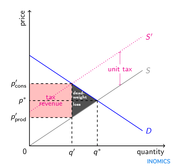
If supply is completely inelastic, there is no deadweight loss. If supply is completely elastic, there is the usual deadweight loss.
Under perfect competition, small firms accept prices from the market and receive no profits. In a monopoly, one large firm sets the price \(p\) at the point where marginal revenue equals marginal cost. Price discrimination allows monopolies to capture all of consumer surplus.
Oligopoly
Game theory is the study of decisions where the payoff of a player \(i\) depends on the actions of another player \(j\). A set of strategies is in equilibrium if there are no positive utility deviations. A Nash Equilibrium always exists in mixed strategies \(\sigma\).
In Cournot oligopy, firms simultaneously choose quantities, leading to pricing above marginal cost. In Bertrand oligopy, firms choose prices and then produce quantities; it suggests that firms should be in perfect competition. In the case of second-price auctions, it is weakly dominant for everyone to bid their value \(v_i\)
Intertemporal
Thus far, we assume time consistency in intertemporal decisions. Suppose that across each period \(t = 0, 1, 2\), agents have income \(M'_i = M_i + \text{savings/debts}\) and choose consumption \(c_i\). Plans for the future coincide with future actions, since we can rewrite the utility function: \(u(c_0, c_1, c_2) = U(c_0) + \frac{1}{1+\delta}[U(c_1) + \frac{1}{1+\delta}U(c_2)] = u(c_1) + \frac{1}{1+\delta}u(c_2)\) But the time consistency doesn’t seem to model addictive products, good actions, or immediate gratification. Instead, we can apply a constant discount rate to all non-immediate utility so that: \(u(c_t, c_{t+1}, ...) = u(c_t) + \frac{\beta}{1+\delta} u(c_{t+1}) + \frac{\beta}{(1+\delta)^2} u(c_{t+2}) + ...\) The FOC is now inconsistent over periods. For \(t=1\), we have \(\frac{U'(c_1^*)}{U'(c_2^*)} = \beta \frac{1+r}{1+\delta}\). But for \(t=0\), we still have \(\frac{U'(c_1)}{U'(c_2)} = \frac{1+r}{1+\delta}\).
We see this in practice for health clubs. People buy long-term contracts as commitment devices, but they overestimate future attendance and delay cancellation.
Final
Oligopoly
Under an oligopoly, only \(p_1 = c = p_2\) is a unique Nash Equilibrium. Neither firm has an incentive to deviate, and for any other case, at least one firm can profitably deviate.
Under Cournot oligopoly, firms choose quantities. Under Bertrand oligopoly, firms choose prices and then produce the quantity demanded by market. Bertrand Competition thus concludes that just two firms guarantee perfect competition, whereas Cournot oligopolies produce above the marginal cost. In a Stackelberg oligopoly, one firm makes the quantity decision first.
Suppose we have cost \(c(y) = cy\) with demand \(p(Y) = a-bY\). Under monopoly, we have \(y_M = \frac{a-c}{2b}\) and \(p_M = \frac{a+c}{2}\). Under Cournot, we have \(Y_D = 2\frac{a-c}{3b}\) and \(p_D = \frac{1}[3} + \frac{2}{3} c\). Under Stackelberg, we have \(Y_D = 3\frac{a-c}{4b}\) and \(p_D = \frac{1}{4}a + \frac{3}{4}c\).
Auctions
In second-price auctions, each individuals has a private value \(v_i\) and a bid \(b_i\). Through casework, we can show that \(u_i(v_i, b_{-i}) \geq u_i(b_i, b_{-i})\). In other words, betting one’s own value is weakly dominant. However, in the real world, users of eBay may bid multiple times or overbid.
Dynamic Games
| In dynamic games, one player plays after the other. The second player must always express their strategy in the form of a condition (Choice 2 | Choice 1). We can consider the subgame-perfect equilibriums, where the player chooses the highest-payoff strategy given the other players’ strategy. Dynamic games can enable some cooperation. |
Edgeworth Box
An edgeworth box involves two consumers \(i = a, b\) with two goods \(x_1, x_2\) where each consumer \(i\) has an endowment \(\omega^i_j\) of good \(j\). We denote total endowment \((\omega_1, \omega_2) = (\omega_1^a + \omega_1^b, \omega_2^a + \omega_2^b)\).
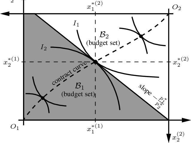
The individual rationality condition is satisfied where \(u_i(x_1^{i*}, x_2^{i*}) \geq u_i (w_1^i, w_2^i)\) while Pareto efficiency denotes the optimal utility for all agents. The barter lens is the area that satisfies the individual rationality condition. The Pareto set is the set of points where indifferent curves are tangent; the subset within the individually rational area is called the contract curve.
Suppose both consumers face budget constraints such that \(p_1x_1 + p_2x_2 \leq p_1\omega_1 + p_2\omega_2\)
A Walrasian Equilibrium denotes a point where each consumer maximizes utility subject to their budget constraint. The offer curve for each consumer is the set of points that maximize utility as a function of \(p_1, p_2\). At the intersection of these points, both individuals maximize utility given prices and the total quantity demanded is equal to the total endowment.
An increase in the endowment \(\omega\) increases final consumption. An increase in \(p_2/p_1\) increases \(x_1\) and decreases \(x_2\).
Asymmetric Information
For workers, drivers, and CEOs, the agent’s effort is unobserved, so principal, whether the employer, insurer, or shareholder, has to use a proxy. Agents may get bad luck and be punished, or get lucky and be rewarded for low effort. This is a hidden action or moral hazard.