
Notes: IEOR 160 / Nonlinear & Discrete Optimization
Published:
I took these notes for IEOR 160: Nonlinear and Discrete Optimization taught by Javad Lavaei.
Midterm
Optimality Conditions
Univariate
For a function $f$, a stationary point $x^$ has $f’(x^) = 0$. If
- $f’‘(x^) < 0$, then $x^$ is a strict local maximizer.
- $f’‘(x^) > 0$, then $x^$ is a strict local minimizer.
- $f’‘(x^) = 0$, then consider further derivatives. If the *first nonzero derivative occurs at an odd number of derivatives, then $x^*$ is a saddle point.
Feasibility
Suppose $f$ is only defined on $[a, b]$. A stationary point $x^$ is only feasible if $a \leq x^ \leq b$. To find the global optimum, compare the local optima with the boundaries $a$ and $b$.
Multivariate
For a function $f(x)$ with $x \in \mathbb{R}^n$, stationary points $x^$ have $\nabla f(x^) = 0$. Compute the Hessian $H_f = \nabla^2 f$, where $(H_f)_{i, j} = \frac{\partial^2 f}{\partial x_i \partial x_j}$. If the Hessian is
- negative semi-definite (NSD), then $x^*$ is a strict local maximizer.
- positive semi-definite (PSD), then $x^*$ is a strict local minimizer.
- indefinite (ID), then $x^*$ is a saddle point.
Definiteness
There are several tests for the definiteness of the Hessian:
- Principle Minors. Compute the determinants of each upper left submatrix. If all are positive, then the Hessian is PSD. Vice versa for NSD. If neither, ID.
- Eigenvalues. If all eigenvalues are positive, the Hessian is PSD. Vice versa for NSD, and ID if neither.
- Pivots. Reduce matrix to row-echelon form. Pivots are the first nonzero element in each row. All pivots should be positive/negative for PSD/NSD, respectively.
Approximation
The first-order approximation of $f(x + \delta)$ is:
\[f(x + \delta) \approx f(x) + \nabla f(x)^T \delta\]A second order approximation adds the Hessian:
$f(x + \delta) \approx f(x) + \nabla f(x)^T \delta + \frac{1}{2} \delta^T \nabla^2 f(x) \delta$
Descent Directions
To identify a descent direction for a function $f$ at some point $\bar{x}$, compute the Taylor expansion about $\bar{x}$ and identify the dominant (/first non-trivial) term. Any vector $\delta x$ that makes the term negative is a valid descent direction. An alternative approach is to compute the eigenvalues; a negative eigenvalue corresponds to a descent direction. Vice versa for acsent directions.
Coercive
A function $f$ is coercive if $\frac{f(x) \cdot x}{| x |} \to + \infty$ as $| x | \to \infty$. In other words, $f$ must approach $+\infty$ from all directions.
Numerical Algorithms
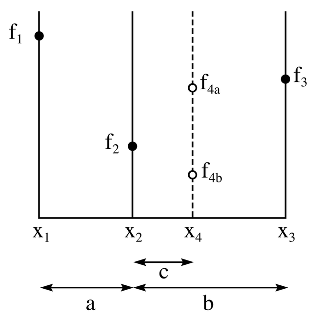
Golden Section
Consider a unimodal function $f(x)$ and an interval $x_1, x_3$. Select a point $x_2$ such that the two intervals $a$ and $b$ have ratio $\phi - 1$:$2 - \phi$, where $\phi = \frac{1 + \sqrt{5}}{2}$. Choose $x_4 = x_1 + (x_3 - x_2)$ to gaurantee $a + c = b$ and a reduction of the interval width by $\frac{1}{\phi} \approx 0.608$.
In general, for an approximation of $f$ over $[a, b]$ to satisfy tolerance $\epsilon$, we need $k$ iterations where
\[k \geq \frac{\log \frac{\epsilon}{b-a}}{\log r}\]Gradient Method
To minimize $f$, a update needs a direction and step size. The gradient method chooses descent direction $\delta = -\nabla f(x)^T$. For the step size, there are two approaches:
- Exact line search, which picks step size $\alpha$ via $\min_\alpha f(x + \alpha \delta)$.
- Backtracking line search, an inexact algorithm, which starts with parameters $\alpha, \beta$ and picks the smallest $m$ such taht $f(x + \alpha \beta^m \delta) < f(x)$.
Newton’s Method
Newton’s method is a second-order version of the gradient method. The descent direction is:
\[\delta = -\nabla f(x)^T + \frac{1}{2} \delta^T \nabla^2 f(x) \delta\]The step size follows the same approach.
Convex Optimization
Convexity
A set $C$ is convex if $\forall x, y \in C, t \in [0, 1]$, we have $z = tx + (1-t)y \in C$.
A function $f$ is convex if and only if $\forall x, f’‘(x) > 0$. Analogously, for a multivariate function $f$, the function is convex if and only if $\forall x, H_f(x)$ is PSD. A function $f$ is concave if $-f$ is convex.
If $f$ is a convex function on a convex set $C$, then any local solution is also a global solution.
Useful principles:
- Linear inequalities are convex (and convex!).
- If $f$ is the sum of convex functions, then $f$ is also convex.
- A linear transformation of a convex set is still convex.
- If $C_1, C_2$ are both convex, then $C_1 \cap C_2$ is convex.
Convex Optimization
Consider a convex function $f$, a set of linear equalities $h_1(x) = 0, h_2(x) = 0, …, h_m(x) = 0$ and convex inequalities $g_1(x) \leq 0, g_2(x) \leq 0, …, g_l(x) \leq 0$.
Classes of convex optmization:
- LP: With a linear objective and linear inequalities, the problem is a linear program that can be solved by checking every vertex.
- QP: If the objective is quadratic and convex with linear constraints, the problem is a quadratic program and the number of possible solution is infinite.
- QCQP: With quadratic constraints, the quadratically constrained quadratic program has form $f = x^T p_0 x + q_0^T x + r_0$ and constraints $x^T p_i x + q_i^T x + r_i \leq 0$.
Constrained Optimization
Consider an objective function $f$ and equalities $h_i$. A point $y$ is considered a regular point if all active constraints $\nabla h_i(y)$ are linearly independent. If $x^$ is a local minimum and a regular point, then $\exists \lambda_i$ such that $\nabla f(x^) + \sum_i \lambda_i \nabla h_i(x^*) = 0$ (stationarity). In practice, often the first step is to verify that no regular points are feasible.
First Order Necessary Condition: For a regular point and local min $x^*$, the Karush–Kuhn–Tucker (KKT) conditions imply $\exists \lambda_1, …, \lambda_m, \mu_1, …, \mu_l$ satisfying:
- Stationarity: $\nabla f(x^) + \sum_i \lambda_i \nabla h_i(x^) + \sum_j u_j \nabla g_j(x^*) = 0$
- Complementary Slackness: $\mu_j g_j(x^*) = 0$
- Dual Feasibility: $\mu_j \geq 0$
- Primal Feasibility: $h_i(x^*) = 0$ and $g_j \leq 0$
Usually, we consider combinations of $\mu_j = 0$ and $\mu_j > 0$.
Second Order Necessary Condition: Let $M = \nabla^2 f(x^) + \sum_i \lambda_i \nabla^2 h_i(x^) + \sum_j u_j \nabla^2 g_j(x^)$. Then, $\delta x^T M \delta x = H(\delta x) \succcurlyeq 0 \iff E^T M E \succcurlyeq 0$, where $E$ is a basis for the tangent plane at $x^$. To select $E$,
The second order condition is sufficient if $x^*$ is non-degenerate ($\mu_j > 0$) and $M \succ 0$. Intuitively, any unconstrained local optimum will also be a constrained local optimum.
Duality
For a primal $\min_x f(x)$ with $h_i(x) = 0$ and $g_i(x) \leq 0$, the dual is: $\max \min \mathcal{L}(x, \lambda, \mu) = \max d(\lambda, \mu) \text{ s.t. } \mu \geq 0$
Non-convex problems have a duality gap $p^* - d^$. A convex problem that satisfy Slater’s condition guarantees convex $\mathcal{L}$, $p^ = d^$, and KKT conditions for $p^, d^*$. Slater’s condition requires a feasible point $y$ that is feasible and strictly satisfies inequalities.
After reformulating the problem in terms of minimizing the Lagrangian, some conditions on $x$ are usually required to prevent a trivial $-\infty$ minimum.
Pertubations
Pertubations of size $\epsilon$ of a solution $f_$ are roughly $f_\epsilon \approx f_ - \sum \lambda_i \epsilon _i - \sum \mu_j \epsilon_j$.
Discrete Optimization
In discrete optimization, we consider $x \in \mathbb{Z}$. Mixed-integer programming mixes real and integer variable. Relaxing the discrete constraint into a continuous constraint yields a lower bound.
Branch-and-bound concieves of discrete optimization as a series of convex optimizations. Relax all constraints and compute the optimum $p$. If $p$ is integer, then $p$ is the optimal solution. Otherwise, pick some $y_i^\text{opt} \not \in \mathbb{Z}$ and branch into $y_i < y_i^{\text{opt}}$ and $y_i > y_i^{\text{opt}}$. Each time we recursively branch, we introduce a new inequality; the solution is the optimon among all leaves.