I took these notes for EECS 16B: Designing Information Devices and Systems II taught by Vladimir Stojanovic and Murat Arcak.

Midterm

Complex

Cheat sheet for complex numbers:

Transistor

The CMOS inverter is comprised of a NMOS transistor and PMOS transistor. A NMOS transistor is on if $V_{GS} = V_G - V_S > V_{tn}$. The PMOS transistor is on if $V_{SG} = V_S - V_G > V_{tp}$.

Differential Equations

For first-order homogeneous differential equations of the form $\frac{\partial}{\partial t} x(t)) = ax(t)$, we guess the general solution $x = ke^{at}$ and solve for $k_0$ via initial conditions. To prove the solution is unique, notice for any other solution $y$, we have $\frac{\partial}{\partial t} y/(k_0 e^{at}) = 0$, so $y = k_0 e^{at}$.

For nonhomogeneous differential equations (where all 0 is not a solution) of form $\frac{\partial}{\partial t} x(t) = ax(t) + b$, we substitute $\tilde{x} = x + \frac{b}{a}$ and solve with the form above.

For the form $\frac{\partial}{\partial t} x(t) = \lambda x(t) + u(t)$, we deploy the general solution $x(t) = x_0e^{\lambda t} + \int_0^t e^{\lambda (t-\theta)} u(\theta) dt$. For example, suppose $\frac{\partial}{\partial t} V(t) = \lambda V(t) - \lambda t^k e^{\lambda t}$ for $t \geq 0$ and $k > -1$ and $v_0 = 0$. Integrating, we have $V(t) = (-\lambda) \int_0^t \theta^k e^{\lambda t} d \theta = (-\lambda)e^{\lambda t} \int_0^t \theta^k d\theta$.

A useful tool for vector diffeq is a change of basis. Suppose we have $\frac{\delta}{\delta t} x(t) = A \vec{x}(t) + \vec{b}$ where $A$ is diagonalizable, so we can rewrite $A = V\Lambda V^{-1}$. Now, defining $x(t) = V\tilde{x}(t)$, we can solve: \(V^{-1} \frac{\partial}{\partial t} x(t) = V^{-1}(V\Lambda V^{-1}) x(t) + V^{-1} \vec{b}\) \(\frac{\partial}{\partial t} \tilde{x}(t) = \Lambda \tilde{x}(t) + V^{-1} \vec{b}\)

Using the new initial conditions $\tilde{x}(0) = V^{-1}x(0)$ to solve and change basis to yield the desired solution.

RLC Circuits

A capacitors and inductors are similar: \(I_C(t) = C \frac{\partial V_C(t)}{\partial t}\) \(V_L(t) = L \frac{\partial U_L(t)}{\partial t}\)

The voltage across a capacitor and current across an inductor cannot change instantaneously.

In series, $I_{C1} + I_{C2} = I_C$. In parallel, $V_{C1} + V_{C2} = V_C$. In series, $V_{L1} + V_{L2} = V_L$. In parallel, $I_{L1} + I_{L2} = I_L$.

Phasors

Often, we can rewrite AC voltage inputs as $v(t) = \tilde{V} e^{j\omega t} + \overline{\tilde{V}} e^{-j\omega t}$, where $\tilde{V}$ is the phasor. Phasors let us define impedance, an AC-equivalent for impedance: \(Z = \frac{\tilde{V}}{\tilde{I}}\)

For resistors, $Z_R = R$. For capacitors and inductors, we can derive: \(Z_C = \frac{1}{j\omega C}\) \(Z_L = j \omega L\)

Filters and Transfer Functions

Some transfer functions work as filters with a cutoff frequency at $|H(j\omega_c) = \frac{\max_\omega |H(j\omega)|}{\sqrt{2}}$.

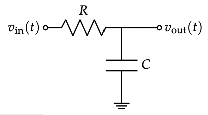
1. The R-C low-pass filter has transfer function $H(j\omega) = \frac{1}{j\omega RC}$ with $\omega_c = \frac{1}{RC}$.

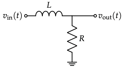
1. The L-R low-pass filter has transfer function $H(j\omega) = \frac{R}{R + j\omega L}$ with $\omega_c = \frac{R}{L}$.

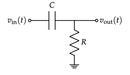
1. The C-R high-pass filter has transfer function $H(j\omega) = \frac{R}{R + \frac{1}{j\omega C}}$ with $\omega_c = \frac{1}{RC}$.

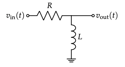
1. The R-L high-pass filter has transfer function $H(j\omega) = \frac{j\omega L}{R + j\omega L}$ with $\omega_c = \frac{R}{L}$.

When combining transfer functions, magnitudes multiply and angles sum. A band-pass filter with $H_{BP}(j \omega) = H_{LP}(j \omega) H_{HP}(j \omega)$.

Control

The state $\vec{x}$ is a collection of a variables which the input $\vec{u}$ can affect. The discrete and continuous models are: \(\vec{x}[i+1] = A\vec{x}[i] + B\vec{u}[i]\) \(\frac{\partial}{\partial t} \vec{x}(t) = A\vec{x}(t) + B\vec{u}(t)\)

Solving the discrete models, we have: \(\vec{x}[i] = A^i \vec{x}_0 + \sum_{k=0}^{i-1} A^{i-k-1} B\vec{u}[k]\)

For a diagonal continuous model, we have: \(x(t) = e^{at}x_0 + \int_0^t e^{a(t-\tau)} \cdot bu(\tau) d\tau\)

If it is diagonalizable, we solve with a change of basis: \(x(t) = Ve^{\Lambda t}x_0V^{-1} + \int_0^t Ve^{\Lambda(t-\tau)}V^{-1} \cdot Bu(\tau) d\tau\)

We can discretize the model by substituting $\vec{u}[i]$, $A_d = Ve^{\Lambda \delta}V^{-1}$, and $B_d V(e^{\Lambda \delta} - I_n)\Lambda^{-1} V^{-1} B_c$.

We model sources of disturbance by adding $\vec{\omega}_c(t)$ or $\vec{\omega}_d[i]$. Disturbances can be ignored or modeled as part of the input.

To identify a system, we feed in test inputs $\vec{u}$ and observe before-and-after states $\vec{x}$. To predict the model $A$, a we can use least squares for matrix estimation, where $P = \begin{bmatrix} A^\intercal \ B^\intercal \end{bmatrix}$: \(\hat{P} = (D^\intercal D)^{-1} D^\intercal S = \argmin_P ||DP - S||^2_F\)

We can apply feedback control by tying $\vec{u}$ to $\vec{x}$ in a way that $A_{CL} = A + BF$: \(\vec{u}[i] = F\vec{x}[i] + \vec{u}_{OL}[i]\) \(\vec{u}(t) = F\vec{x}(t) + \vec{u}_{OL}(t)\)

To assess controllability in a discrete context, we define $C_i = \begin{bmatrix} A^{i-1}B & … & AB & B \end{bmatrix}$. A model is controllable in $i$ timesteps if $\text{Col}(C_i) = \mathbb{R}^n$; a model is controllable if $\text{Col}(C_n) = \mathbb{R}^n$. If a discrete model is controllable, then closed-loop feedback can set all eigenvalues of the closed-loop matrix, a proof which involves a change of basis to controllable canonical form.